Any Excel worksheet that you create can easily become overwhelming, because there's so much information contained in it. For that reason, it's important to learn how to maintain your worksheets to help you keep on top of all the information.

If you're using a small screen – or even an extremely large one – to view data in your spreadsheet, it can be hard to see. This is where the Zoom feature in Excel comes in handy. You can zoom in on a certain area or even a cell.

There are a few ways to use Zoom in Excel. The first is located at the bottom right side of your screen:

You can use the slider to zoom in and out on a worksheet. You can also click on the magnification percentage and enter a new percentage.

Select a new magnification percentage or a custom percentage:

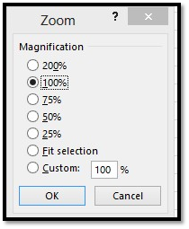
Click OK.

You can also go to the Ribbon and the View tab.

Go to the Zoom group.

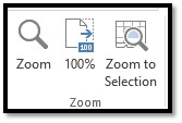
Click the Zoom button.

When you do this, you'll see this dialog box:

Select your magnification, then click OK.

If you click the 100% button on the Ribbon, Excel will show your spreadsheet with 100% magnification.

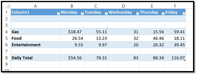
To use the Zoom to Selection button, first select a cell or an area in your worksheet that you want to zoom in on. Then click the Zoom to Selection button.

This is what happens:

As you can see, Excel zoomed in on the selected cell.

You can also take advantage of Excel's different worksheet views to view your data. The views are located to the left of Zoom at the bottom right side of your window.

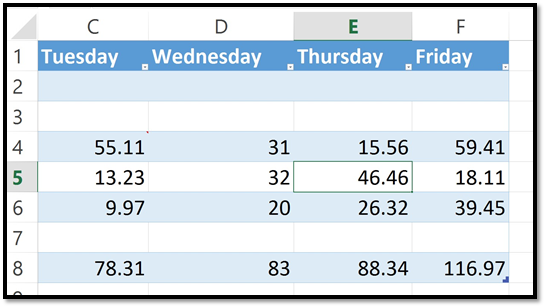
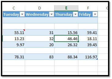
The first view (on the left) is Normal view. This is how we are viewing our spreadsheet right now.

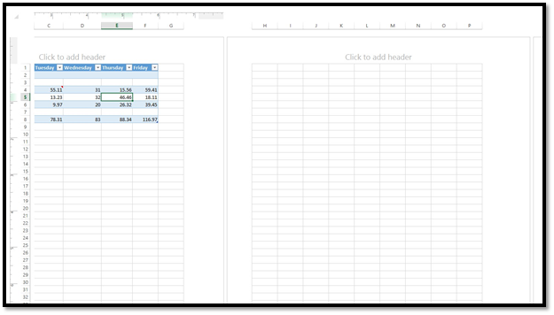
Next is Page Layout view (shown below).

The third one is Page Break view.

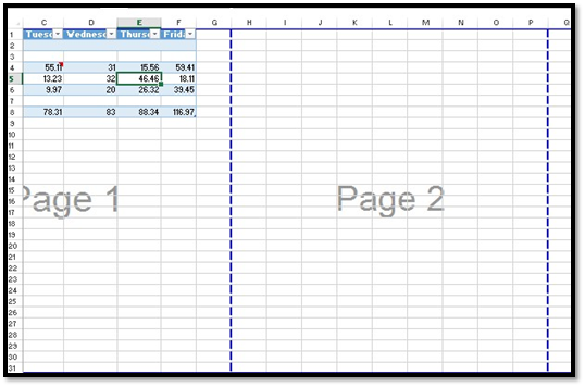
If you're getting ready to print pages or want to see how the layout looks, using these different views can help.

You can use the Research task pane to search for information online using sources such as Bing, the Encarta Dictionary, a thesaurus, and other sources. This can be helpful when you need to do research to complete a worksheet.

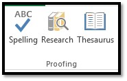
To use the Research task pane, go to the Review tab, and click the Research button in the Proofing group.

A pane will open on the right side of your screen:

Next, type what you want to research in the Search For box. Then choose where you want to search for it in the next section.

You can choose to look in All Reference Books, which will search all dictionaries and thesauri that it has to use. Or you can choose All Reference Sites, which includes Bing.

It's possible that you might create a workbook that contains dozens of worksheets. Let's say, for example, that you create a workbook that contains expense reports for employees. Each employee might have their own worksheet in the workbook. If you have two dozen employees, then you have a lot of worksheets to keep track of and maintain. That, in itself, may not be a big deal, but finding the worksheet when you need it can get tricky.

For that reason, you can have dozens of worksheets within a workbook, but you can also create workbooks for individual worksheets. That way, the data is easy accessible when you need it.

Navigating Between Worksheets

Again, if you have a lot of worksheets, navigating between them can get tricky. Plus, not all the sheets show at the bottom left side of your page.

To easily navigate between sheets, right-click the tab scroll to the left of your worksheets:

When you right click, you'll see the Activate dialog box.

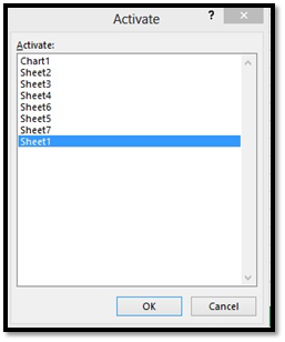
Choose the worksheet you want to activate, then click OK.

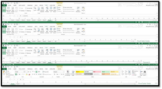
You can display worksheets within a workbook as different windows to make it easier to compare data. That way, you can have more than one worksheet displayed at a time.

To do this, select the worksheet you want to view in a new window.

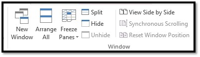
Click the New Window button under the View tab.

When you have multiple versions of one workbook open in several windows – each displaying different worksheets -- you want to be able to arrange the windows so you can view them all at once.

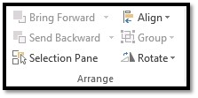
Click the Arrange All button (pictured below).

You'll then see this dialog box:

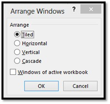
Choose an arrange option.

• Tiled will make it so all the windows fit side by side on the screen.

• Horizontal will make it so the worksheets are placed one above the other.

• Vertical will place them next to each other.

• Cascade will arrange them so they overlap with only their title bars showing.

Put a check beside Windows of Active Workbook to only have windows of the currently active workbook arranged.

We chose horizontal:

To compare two worksheets side by side, click the View Side by Side button.

This will let you compare any two worksheet windows that you have open.

You can also move or copy one worksheet from one workbook to another workbook.

To do this, open the workbook with the worksheet you want to move. Also open the workbook that you want to use to add the worksheet.

Now, go to the workbook with the worksheet you want to move. Click the worksheet so it's active.

Right-click on the sheet tab of the worksheet you want to move. Select Move or Copy from the menu.

In the dialog box, select the name of the workbook you want to move the worksheet to. At this point, you can also select New Book to create a new workbook.

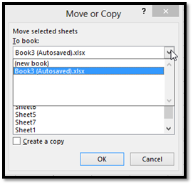
Then select where you want to place it in the other workbook.

Click OK when you're finished.

Adding Images and Graphics

You've already learned how to format a worksheet and enter information into Excel; now we're going to show you how to add elements such as graphics and images.

You can enter these elements into Excel simply by associating them with a particular piece of information. For instance, if you were creating a catalogue of items in a museum, you might want to include a picture of the item next to its description. But you can also use them to make your projects more visually appealing.

You can add images into MS Excel from a file, or directly from a scanner or camera. We'll show you how to add an image stored on your computer first.

To do this, select the cell that will represent the top left corner of your picture.

Next, go to the Insert tab and click Picture.

A dialog box is displayed that allows you to search your computer for the image you want to use.

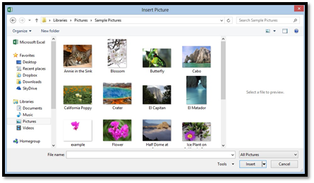
Navigate to the folder that contains the picture you'd like to insert, select the picture, and double-click it, or click Insert.

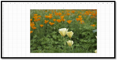
The image now appears in your spreadsheet:

When you insert a picture into Excel, the Picture Format tab automatically opens in the Ribbon. This tab contains the tools you'll need to modify an image or element. We'll talk about it more later on in this section.

You can also insert pictures from memory cards and external devices hooked up to your computer. Follow the same steps and locate the device, then navigate to the picture you want to use.

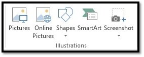
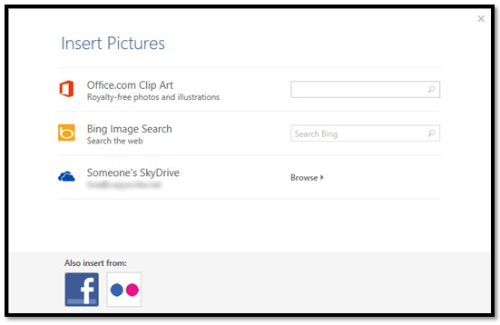
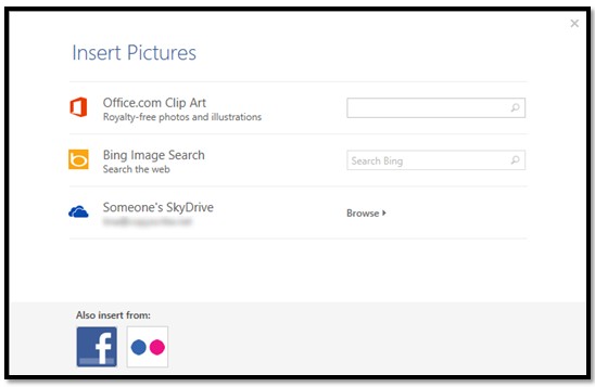
You can also insert MS Office clip art, images you find using a web search, and images from your SkyDrive into a spreadsheet. To do this, click the Online Pictures button.

When you click the button, this window will appear:

If you want to search for Clip Art, type in a description of what you're looking for. Use keywords, such as coffee, woman, shopping, etc.

We're going to type in coffee.

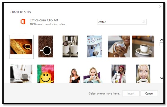
Select the picture you want by clicking on it, then click Insert.

To search for a picture on the web, then insert it into your spreadsheet, type in a keyword just as you did above.

We'll do coffee again.

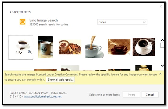
As you can see above, Microsoft lets you know the images shown are licensed under Creative Commons.

As defined by Webopedia:

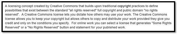
Make sure you check the copyright to be sure you can use the image. To avoid copyright issues, either use your own images, images that are in the public domain (no copyright), or purchase images from stock photo sites where you will receive a license with the image.

In addition to inserting pictures from Bing search, you can also insert pictures stored on your SkyDrive.

Click Browse.

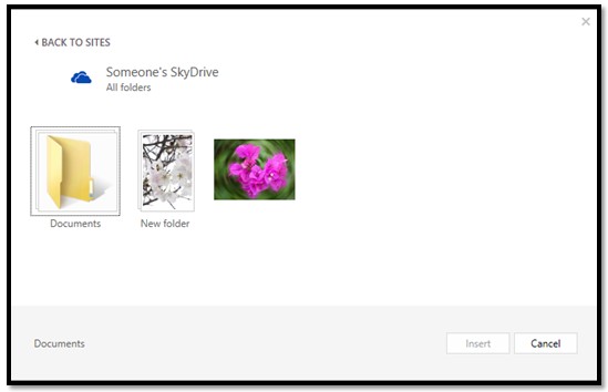
Find the image you want, then click the Insert button.

To insert images from Facebook or Flickr, click the Online Pictures button again.

For Facebook, click the Facebook icon at the bottom of the window.

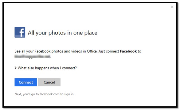
Click Connect.

You'll then be prompted to sign in to your Facebook account:

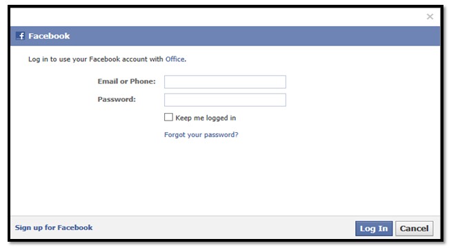
Click Log in. Once you're logged in, you'll see this screen:

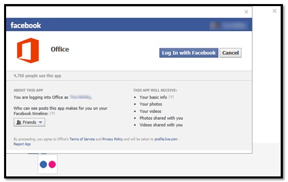
Click Log In with Facebook.

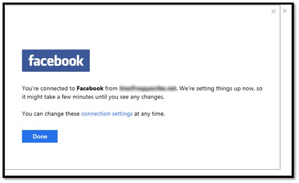
Click Done.

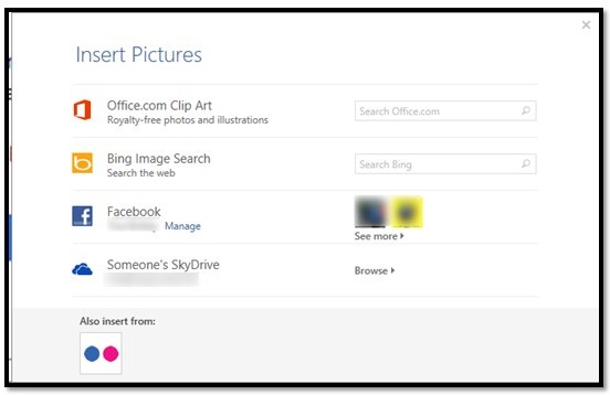
You'll then see Facebook listed with all the other locations where you can search for pictures:

If you want to add pictures from Flickr, click the Flickr button at the bottom to connect to your Flickr account.

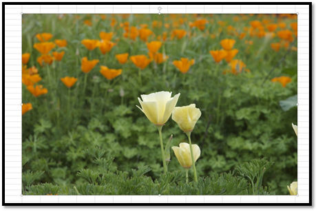
When you crop a picture, you cut away the outer edge of the picture to create a new version.

Let's crop the picture below.

Go to the Picture Format tab (double click on the image if you don't see it) and click Crop from the Size group.

Your cropping options are now displayed in the drop-down menu.

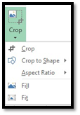
Crop allows you to crop edges away from the image. This is the most commonly used option. You can play with the other ones to see if they work for you. Working with images is mostly about creating the look and style that you want for your spreadsheet.

We're going to select Crop.

As you see above, there are now black crop handles at each corner of the image and halfway across each edge. These crop marks look like "L" and dashes.

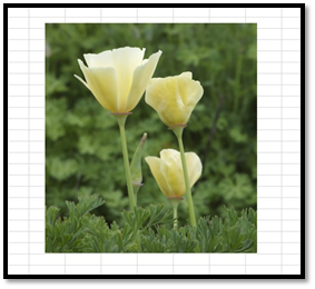
Click and drag your mouse on any of these marks. Click and drag inward on the image until you have cropped away the area you want to get rid of in the image.

The area you're cropping away is shaded in dark gray.

Click outside of the image to remove the cropped area.

You can easily adjust the color of any image you place in your spreadsheets.

To do this, double click on the image.

You'll then see the Picture Tools Format Tab. Click the Color button:

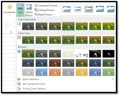
Choose the color effect you want to apply to your image.

Color Correction

You can also adjust and modify the colors in your image through color correction. Once again, go to the Picture Tools Format tab by double clicking your image.

Click the Corrections button.

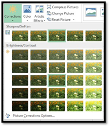
Choose a color correction.

Just as you can use Photoshop and other photo editing software programs to add effects to your images, you can also use Excel for this.

Double click your picture to bring up the Format tab, then click the Artistic Effects button.

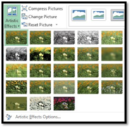
Choose the artistic effect that you want to apply to your image.

To rotate an image, we click the Rotate button in the Arrange group under the Picture Format tab.

Decide how you want to rotate it by making a selection in the drop-down menu:

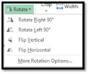
We're going to Rotate Right 90 degrees.

Excel rotates the image for us.

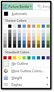
Changing the Borders of a Picture or an Image

The picture border tool is located in the Styles group on the Picture Format Ribbon. Border refers to the border around the outer edge of a selected element. To change the border of an image, you can click this button in the toolbar, and then select the desired weight (thickness) of the line. You can also change the border style in the Colors and Lines tab of the Format picture dialog box. Using this method, you can also easily change the color and style of the line as well.

In addition to adding borders to images, you can also add a style. A style can give the image a 3-D effect, add borders, shadows, and reflections.

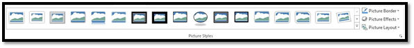
To add a style, select the image, then choose a style from the Pictures Style gallery under the Picture Format tab.

Re-size images using the Picture Tools Format Ribbon.

Go to the Size group and enter a size in images.

You can also re-size a picture by dragging in or out on its handles on the bounding box.

To move an image, click on the image so it's selected. Move your mouse cursor over the image. The cursor will turn into two arrows that look like a plus sign. Now, drag your image to its new location, then release

You can reduce the file size of a picture by using the Compress Picture command. This reduces the resolution of the picture for quicker downloading and removes unnecessary information. For instance, when you crop a picture, the cropped portions of a picture are still stored in the file, they have only been "hidden."

The Compress Picture button is located under the Picture Format tab in the Adjust group.

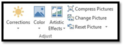
Click the Compress Picture button.

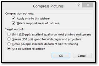
Choose the options you want, and click OK. The e-mail option reduces picture resolution to 96 dpi, or dots per inch. This helps increase the send/receive speed of your spreadsheet when you email it.

Use the Reset Picture button on the Picture Format ribbon to reset the picture to its original size and format.

You might be familiar with WordArt from Excel's sister program Word. You insert WordArt into Excel much the same as you insert a picture.

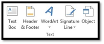
Go to the Insert tab and select WordArt from the Text group.

You will then see the WordArt gallery.

Select a style by clicking on it.

Click inside the box on your spreadsheet to type in your own text.

When you add WordArt, the Drawing Tools Format tab opens in the Ribbon.

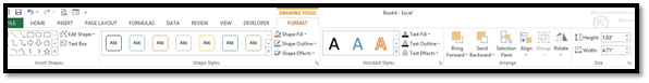
From here, you can format your WordArt by applying a style, fill (the inside coloring of the letters), shape outline (the outline color of the letters), and even effects. These are the same effects you can apply to images.

There are so many things that you can do to customize your Excel spreadsheet. One of those things is adding shapes.

To add a shape, go to the Insert tab and click the button in the Illustration group.

Select a shape from the drop-down menu.

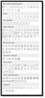
Select a shape. We've selected a cloud in the Callout section. Now simply click in the spreadsheet where you want the shape to appear:

You'll see a bounding box around the shape:

The little arrow at the top of the shape that looks like the Redo sign can be used to rotate the shape to the left or right.

You can drag on the handles (the little squares) to enlarge or reduce the size of the shape.

Double-click the shape to bring up the Format tab on the Ribbon:

A hyperlink is a link to a website or location on the Internet – or even your computer, if the person reading your spreadsheet has access to your computer files. To insert a hyperlink into a spreadsheet, go to the Insert tab, then the Links group. Click the Hyperlink button.

You'll see this window:

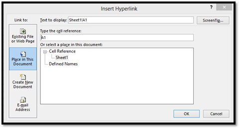
In the Text To Display field, enter in the text you want displayed in your spreadsheet. This will be the text people can click on to take them to the web page. It doesn't have to be a URL. You can type in the word "cow" if you want.

Choose what you want to link to. We've chosen a place in the spreadsheet.

Click OK when you're finished.

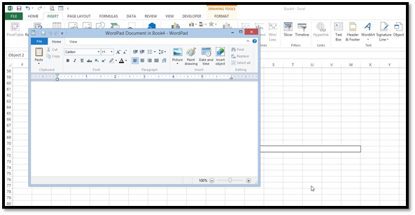
To embed an object into Excel, select a location, then click the Insert tab, then the Object button.

The Object dialog box will open.

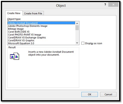
As you can see, you can now choose an object to embed. We're going to scroll down and embed a WordPad document.

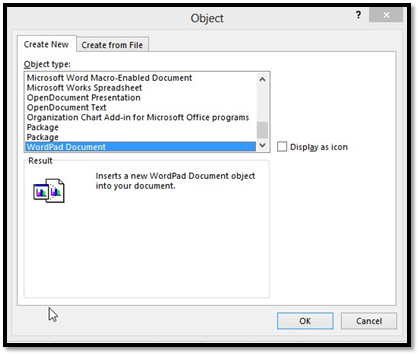
Click OK when you've chosen your object.

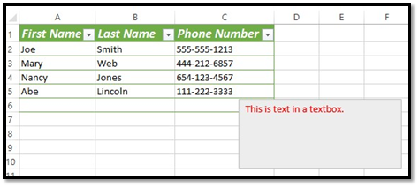
We now have a WordPad spreadsheet open on top of our spreadsheet. If you look to the right of the WordPad document, you'll notice a text box where your text will be placed.

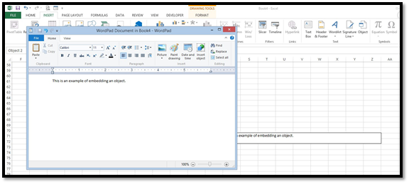
Start typing into the WordPad document.

When you're finished, click the File tab in the WordPad document.

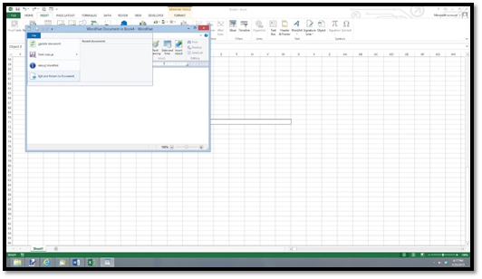
Select Exit and return to document.

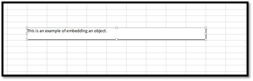
The object is now embedded. You can re-size, move, and even format the object.

To create a text box, go to the Insert tab and find the Text box button in the Text group.

Click the Text Box button.

The cursor changes to a downward arrow over your spreadsheet.

Simply click and drag to draw your text box. You do not have to draw it according to cells. In other words, you don't have to worry about starting at the top corner of one cell and dragging. You can put it wherever you want.

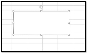
When you quit dragging and release your mouse, the cursor will appear in the text box.

Enter your text.

You can format the text in a text box the same way that you format a cell.