A pivot table sounds more difficult and confusing than it really is. Most people say they don't like pivot tables, or they don't understand them. In truth, they're not that difficult at all.
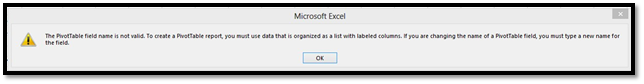
Before you can create a pivot table, you must create a data list with labeled columns. Otherwise, you will see this message:
The best way to learn about a pivot table is to see how to create one.
We've created the table shown below. In tables, columns are fields and rows are records.
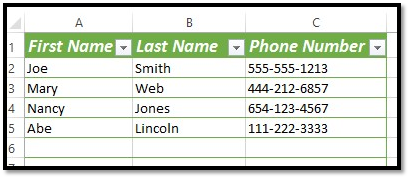
We want a pivot table showing us how many phone numbers are on file for each employee.
To do this, select the table, then go to the Insert tab and click Pivot table.
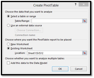
The Table/Range is selected for you. Select New Worksheet, then click OK.
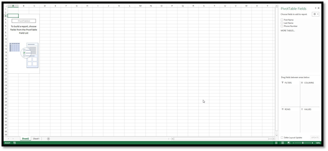
On the right, you'll see the Field list open up. This is a list of all fields in your table.
There are three kinds of fields:
-
Category fields are fields that you can group. In ours, we grouped category fields by department and position.
-
Data fields are fields that contain data that you can add, subtract, multiply, or divide. In ours, that's the salaries.
-
Arbitrary fields are fields that are neither data or category. The name field in our table would be arbitrary.
This is what you should now see on your screen:
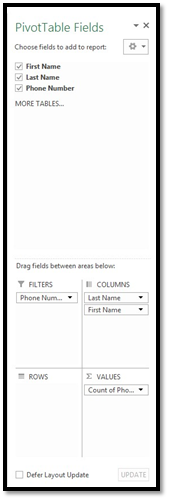
If you look at your Pivot Table Field list on the right, you can drag and drop from the "Choose Fields to Add to Report" section down to the "Drag Fields Between Areas Below" section. Just drag and drop from the top part of the field list to the bottom part and place it in a category: Filters, Columns, Rows, and Values.
Your pivot table will appear in your spreadsheet as you do this. You can always drag and drop to a different section if you want.
Here's what we've done in the Field list on the right:
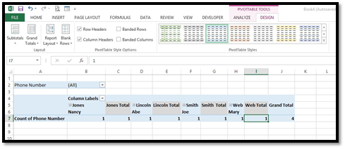
Look at what that's created.
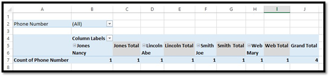
Now we can see how many phone numbers we had for each person. We can also use the filter we created at the top to select a phone number to find out who it belongs to. You can add a filter for any category: First Name, Last Name, or Phone number (in the case of our table).
Here's a better example because it shows you what a pivot table can do with your data.
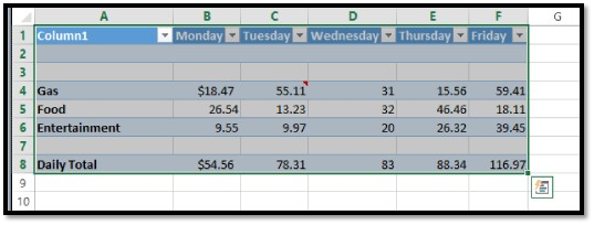
Below is our table.
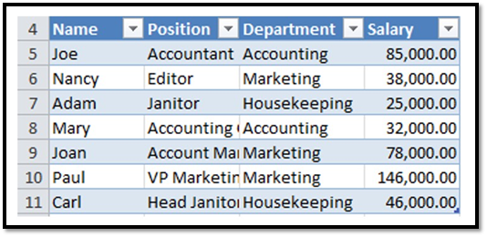
Let's create a pivot table using the table above.
We want Position to be a Row Header, so we drag and drop to Row Labels. We want the values shown in the table to be salary, so we will drag and drop that to Values.
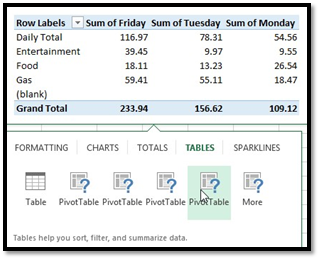
Look at what that's created.
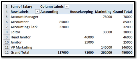
Now we can see the salary by department and by job description. If we had more than one salary per job description, it would total the salaries for us. Let's amend the chart to show you what we mean by adding another Account Manager.
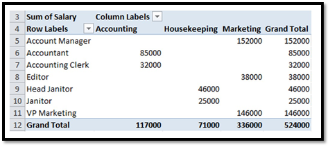
As you can see, we added another Account Manager to our table.
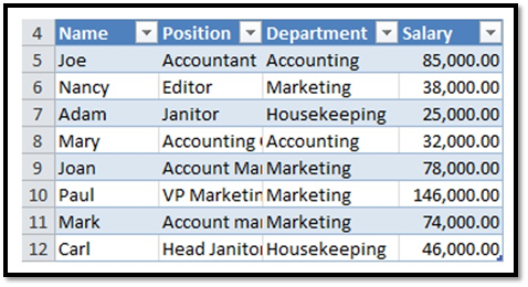
The totals in the pivot table reflect both salaries.
Tip: Make sure there aren't blank rows or columns before you begin. Otherwise, Excel will only create the pivot table/chart up to the blank row or column.
A quicker way to create a pivot table is using the Quick Analysis tool. To do this, select the data in a table that you want to use to create a pivot table.
The Quick Analysis tool button appears at the bottom right, as shown below.
Click the button and choose Tables.
Now, mouseover the PivotTable buttons to choose the pivot table that you want.
Formatting a Pivot Table
You can format a pivot table just as you would any other table.
To format a pivot table, click within the pivot table.
Then, click on the Pivot Table Tools Design tab.
You can choose a layout for the table, as well as a style.
Filtering Using Data Slicers
When we created a pivot table, we added a filter when we created the table. We can also, however, add a slicer to the table. A slicer will filter your data too. You just select the data you want in each slicer.
Let's show you what we mean using our first table as an example
Go to the Pivottable Tools Analyze tab, then go to the Filter group, as pictured below.
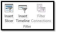
Click the Insert Slicer button.
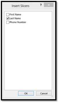
As you can see above, we chose Last Name.
Click OK.
Excel adds the slicer as a graphic object. You can move and format it as you would any other graphic object.
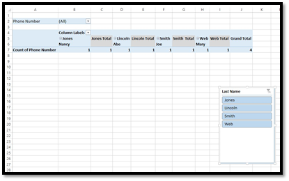
As you can see above, the slicer contains only the data that we selected.
You can also create a pivot chart from a table.
Click the Pivot Chart button under the Insert tab. Select if you want to create just a pivot chart � or a pivot chart and table.
We're going to just create a pivot chart.
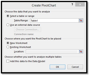
Select the table or range.
Next, select if you want it in a new or existing worksheet.
Click OK.
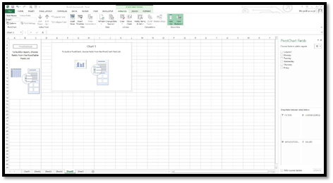
Now you can organize your pivot chart just as you did a pivot table. The only difference is you have two different categories: the axis and the legend.
Changing Field Settings for Pivot Tables and Pivot Charts
When creating pivot charts and tables, you may want to modify the fields listed in the Field list on the right so that the data that you want displayed is displayed in your pivot chart or pivot table.
To show you how to do this, let's refer back to our pivot chart in the last section. In the Values section in the Field list, we notice that it's showing a count instead of totals. We want totals displayed.
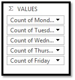
To change this to totals, click the downward arrows, then select Value Field settings.
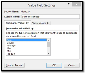
We've selected SUM.
Click OK.
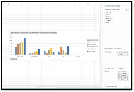
Below is our pivot chart. You can see the Field list to the right.
Headers and Footers
Headers appear at the top of a worksheet. Footers appear at the bottom. Both can contain page numbers, and headers often contain the title of the worksheet, and perhaps the date.
To insert a header or footer, go to the Insert tab and choose Header & Footer.
Click the Header & Footer button. This is what you'll see in your spreadsheet:

When you add Headers & Footers, Excel takes you to Page Layout view.
Also, when you add a header, the Header & Footer tools appear in the Ribbon.
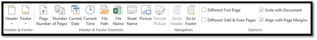
As you can see above, you can add page numbers, number of pages, date, time, sheet name, a picture, etc.
We just added text.
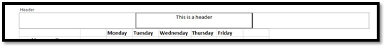
Click outside of the header to apply it to your worksheet.
Now, you can scroll down your worksheet to add a footer:
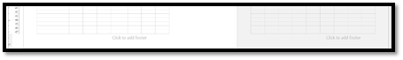
Click to add the footer.
Here we're going to add the page number.
This is what you'll see:
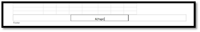
Click outside of the footer area, and your page number is added:
When you're finished adding headers and footers, go to the View tab, then click Normal view to exit out of Page Layout view.
When you're finished creating the worksheets in your workbook, you may want to print them out. Printing in MS Excel is very easy. Excel makes it that way. To print your workbooks and worksheets, click the File tab to get to the Backstage area.
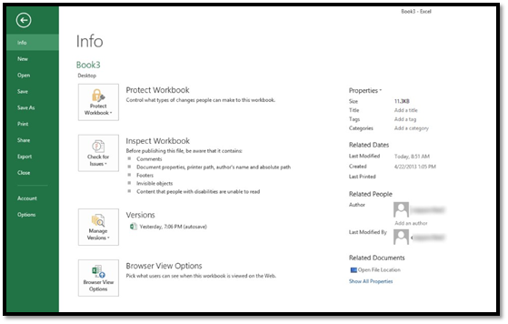
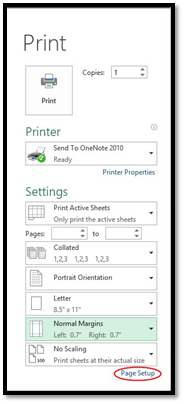
Click Print on the left.
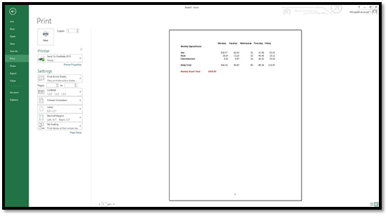
On the left side, you'll be able to set your print options.
On the right side, you'll see the print preview.
To prepare your workbook or worksheets for printing, first select your printer in the Printer section on the left.
Then, specify your settings.
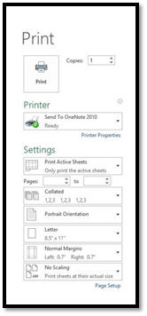
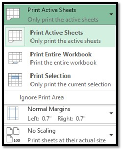
Under Print Active Sheets, select what parts of your workbook you want to print. This allows you to print all, or just portions, of your file. You can choose:
-
Print Active Sheets to print the worksheet that is currently active (or being displayed) in Excel.
-
Print Entire Workbook to print all worksheets in the workbook.
-
Print Selection to print just the cells you have selected.
Under Collated, you can select how you want multiple copies to print. For example, let's say you print 10 copies each of Sheet1 and Sheet2. Do you want the printer to print 10 copies of Sheet1 first, followed by 10 pages of Sheet 2? Or would you prefer to print Sheet1, Sheet2, then Sheet1, Sheet2, etc., until then copies have been printed?
Next, decide if you want to print in Portrait (the shortest side of the paper is horizontal) or Landscape (the longer side of the paper is horizontal) orientation.
Finally, select Paper Size, Margins, and whether you want to print the worksheets at their full size, or scale them down to smaller sizes to fit easier on paper.
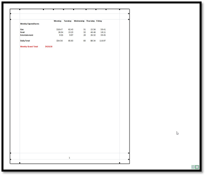
Now, let's look at the right side of the Print screen � or the print preview. In the right bottom corner, you'll see these two icons:

The first icon (from left to right) is the Show Margins icon. When you click this, Excel will show you the margins in Print Preview as you have them set:
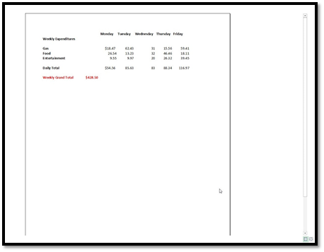
The next icon is Zoom to Page (highlighted). This shows you the active worksheet as it appears at 100 percent magnification.
You can flip through to view other worksheets by either entering a page number, or pushing the back or forward arrows located in the left corner of the print preview area:

Margins are the space around all edges of your spreadsheet when you print it. It's just the same as if you print a document or anything else.
To set margins, first select the worksheets you want to print by clicking on the File tab, then clicking Print. We already covered print settings.
To set margins, click on the downward arrow beside Normal Margins.
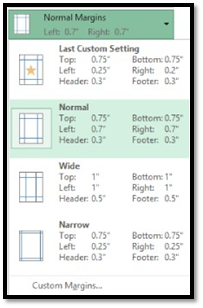
You can select one of the pre-defined margins, or click Custom Margins to customize your margins:
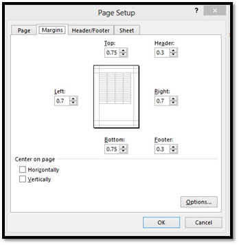
In the Top, Left, Right, and Bottom boxes, enter the margin size you want. Margins are measured in inches.
If you want to center the page vertically or horizontally, you can check either box below the Center on Page section.
In the same dialog box as pictured above, you can also set margins for your headers and footers.
To enter a new distance from the top of the page to the header, change the number in the header box.
Note: Do not switch over to the Header/Footer tab.
To enter a new distance from the bottom of the page to the footer, change the number in the footer box.
When you're finished, click OK.
Selecting the print area simply means you will define the parts of the spreadsheets and workbooks you want to print. If you do not wish to print an entire workbook or an entire spreadsheet, you'll need to do this.
To do this, click on the File tab, then Print.
Page Setup is a text link at the bottom of your print options, as circled in red below:
Click on Page Setup, then click on the Sheet tab in the dialog box.
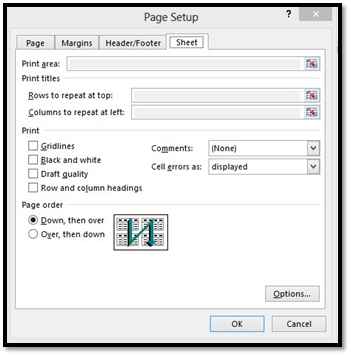
In the Print area box, select the range of cells you wish to print. For example: A1: B10. This would print all cells in columns A and B, and rows one through 10.
In the Print titles section, you'll set the row you want to set as a title. If it's row 1, you would type $1:$1. This row will print at the top of every page. You could also type $1:$2 to print rows one and two at the top of every page.
For columns that you want to appear on the left of every page, type, for example, $A:$C to print columns A through C on the left of every page in the Columns to repeat at left box.
In the Print area, you can select preferences, including if you want the grid lines to appear on your printed worksheet.
Using the Page order section, you can tell MS Excel 2013 in which order to print your sheets.
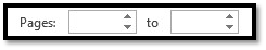
If you don't want to print the entire worksheet, you can set the pages you do want to print.
Click the Print Active Sheets under Settings in the Print section of the Backstage area. We already talked about this earlier. Here you can print active sheets, the entire workbook, or a selection.
Below this box, you'll see Pages. You can enter the pages that you want to print. The pages must be within a range. For example: pages 2 through 5.
To print your MS Excel 2013 workbooks and worksheets, click the File tab, then after all your options are set, set the number of copies you want and click the Print button.