Changing Column Width
In MS Excel 2013, the width of a column is determined by how many characters can be displayed within a cell.cours
To set a column to a specific width, select the column you want to format.
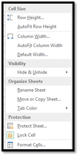
Next, go to the Cells group under the Home tab. Look for Format.
Click the drop-down arrow below Format:
Select Column Width.
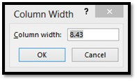
Type in the width of the column, keeping in mind that it reflects the number of characters that can be displayed.
Maybe you just want to make sure the columns are wide enough to display all the contents, but you don't want to take the time to count characters. Perhaps you aren't even sure how many characters there will be, but want to make sure the column will be wide enough, anyway.
Go back to the Format drop-down menu. This time select AutoFit Column Width.
Select the column whose width you want to match.
Copy the column by right-clicking and selecting copy.
Next, select the column whose width you want to change. Right-click within a cell in that column and select Paste Special.
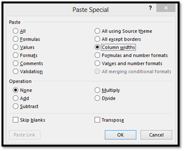
Put a check by Column Widths, then click OK.
To change a default column width for a worksheet, click the worksheet tab to make the worksheet active. To change it for the entire workbook, click a worksheet tab, then right click, and select Select All Sheets.
Now, go back to the Home tab and click the Format drop-down arrow again.
Select Default Width.
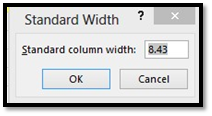
In the Standard Width box, type the new measurement.
To change the width of one column using your mouse, drag the right side of the column to the right until you reach the desired width. To do so, move your mouse to the line separating two columns until you see horizontal arrows appear.
To change the width of multiple columns, select the columns that you want to change, then drag the right side of one column to its desired width.
To change the width of all the columns in a worksheet, select the entire worksheet by clicking the box to the left of Column A and above Row 1, then dragging the boundary of any column.
You follow the exact same steps to change row height as you did for columns.
To change a row to a specific height, select the row(s) that you want to change.
Go to the Home tab and click the drop-down arrow below Format.
Select Row Height.
Select the row(s) that you want to change.
Select AutoFit Row Height from the Format drop-down menu on the Ribbon.
Drag the boundary below a row to adjust its height. To adjust the height of multiple rows, select the rows, then drag the boundary of one of them.
Working With Formulas and Functions
Introduction to Functions
A function in Excel, by definition, is a pre-designed formula that performs a certain calculation. This can make it easier because you don't have to construct every formula yourself. Whenever you use a function, you only have to supply the values the function will use. The values that you supply are called arguments of the function. Excel does the rest for you.
Functions, just like formulas, always begin with an equal sign (=). After the equal sign, you enter in the name of the function. It doesn't matter if you enter it in uppercase or lowercase. Then, after the name of the function, you provide the arguments of the function. Enclose these in parentheses.
There are just a few things you need to remember before starting to insert functions into your spreadsheets:
-
When typing a function into a cell, don't insert spaces between the equal sign, function name, and arguments.
-
If you're adding more than one value, separate each value with a comma.
Below is an example of a function we typed into a cell:
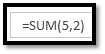
The function was SUM. The arguments were 5 and 2. We hit Enter, and Excel calculated the function for us:

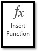
To insert a function directly into a cell, click the cell where you want to insert the function. Next, go to the Formulas tab, then click Insert Function.
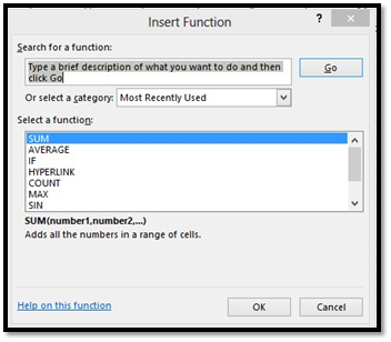
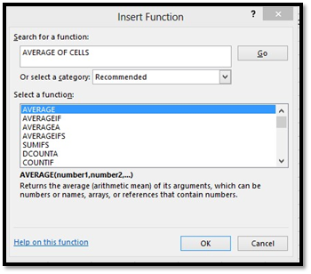
When you click Insert Function, you'll see this dialog box:
In the Search for a Function section, you can type in a description of what type of function you want to use. We typed in Average of Cells. Click Go.
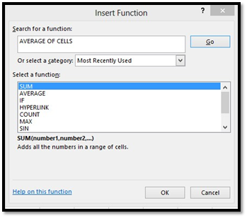
Excel then provides a list of functions that relate to what you were looking for:
In the Select a Function section, you can click on different functions to see what calculations they perform. There are so many different functions in Excel, it's impossible to list them all.
For this example, we're just going to use Average.
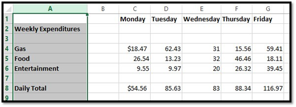
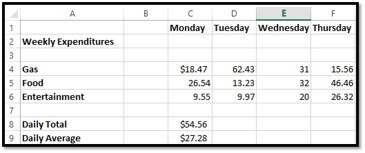
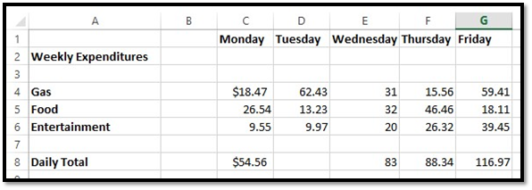
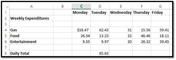
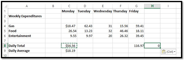
We're going to average Monday's daily expenses in the spreadsheet below:
Now, Excel prompts us for our arguments. We use the cell range C4:C6.
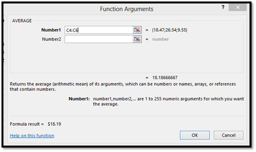
Click OK when your values are added.
As you can see, the average daily expense for Monday was entered into C9.
You can also insert a function by clicking on the Formula Bar.
In the Editing group under the Home tab on the Ribbon, you'll see AutoSum. This is a magnificent little tool that you'll love.
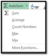
It can also select the most likely range of cells in a column or row that you want to use as the argument, then enters them for you.
You don't have to do anything to use the SUM feature of AutoSum but select the cell. If you want to use AVERAGE, COUNT, MAX, or MIN, you need to select them from the drop-down menu pictured above.
Let's learn to use AutoSum to do a Sum.
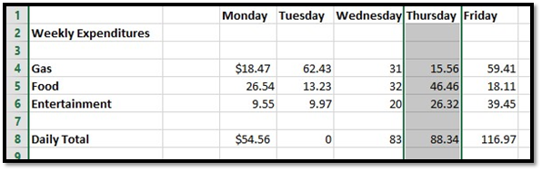
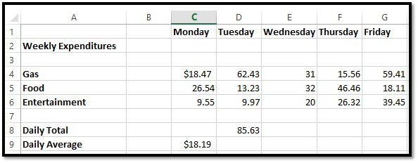
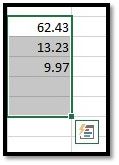
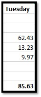
In the worksheet below, the total for Tuesday is missing.
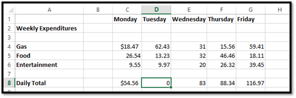
We want the total for Tuesday to appear in cell D8, so we're going to click on the cell.
Now, go to the AutoSum button and click on it.
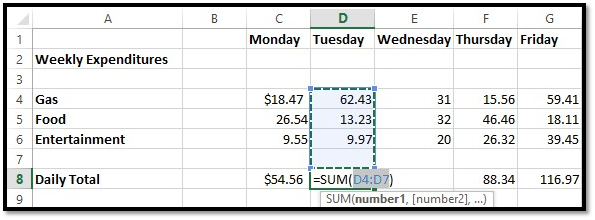
Excel automatically selected the range of cells we want to use in the argument, then entered the arguments into our function.
Hit Enter.
The total was added for us:
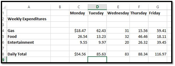
If you want to edit the argument before pushing Enter, you can do that.
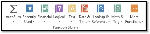
Finding the function you need can seem a daunting task. Of course, you can insert a function by using the Ribbon or Formula Bar, but you can also go to the Function Library under the Formulas tab.
In the Function Library, functions are broken down into categories.
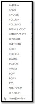
Let's say we want to look for a function in Lookup & Reference.
Click the downward arrow. You'll see all the functions that you can use under this category:
You can click on any one of the functions, and the arguments dialog box will appear so you can enter your arguments.
You can also click Insert Function at the bottom of the drop-down menu.
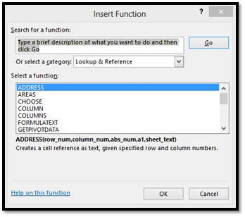
All the Lookup & Reference functions are displayed. Choose the one you want, and click OK.
Quick Analysis is another new feature to Excel 2013. With Quick Analysis, you can do many things, such as adding conditional formatting, charts, pivot tables, and sparklines to your worksheets. It can also add totals to worksheets without you having to use AutoSum.
Let's show you how it works for sums. Once again, we want to calculate the total for Tuesday.
Start by selecting the cells you want to use. We are going to select D4 through D8, because we want the total to appear in D9.
The Quick Analysis tool is shown at the bottom right corner of your selection.
Click on it.
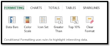
You can see the different categories for Quick Analysis at the top: Formatting, Charts, Totals, Tables, and Sparklines.
Click Totals.
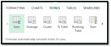
Select Sum.
Quick Analysis calculates the sum and enters the data for you.
A reference simply tells MS Excel where to find the information you want to use in a formula. As you've already learned, by default MS Excel uses the A1 reference style, or coordinate system, to identify cells. You can use these coordinates for references, or you can use labels and names.
Using labels and names makes it easier to understand the information you are entering into the formula. For instance, the formula "=SUM(WednesdayTotal)" is easier to understand than "=SUM(E4:E6)
As you learned earlier, a label is used to identify a range of cells, such as a column or a row. You can also create a name to represent a cell, or a range of cells, for quicker reference in a formula. Names can also represent an unchanging number (called a constant), or even a formula. For instance, let's say sales tax is 8 percent. Since this number will not change between worksheets or workbooks, we can give it a name. In this case, we'll call it SalesTax.
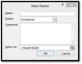
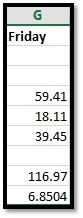
In the snapshot below, we want to name the column Friday as "Friday." This way, when constructing formulas, we can simply enter in Friday instead of a range of cells.
To do this, we're going to select the column "Friday."
Next, we go to Formulas tab in the Defined Names group.
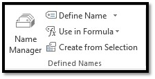
Click the drop-down arrow beside Define Name.
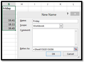
We want the name to stay the same as our label (Friday.) If we didn't, we'd enter a new name, the scope (if we want it to apply to the entire workbook, or just the worksheet), then any comments we want to add.
Click OK.
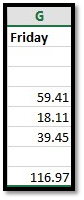
Now we've named this column.
As you can see below, instead of having to write out the formula as =SUM(G4:G6), we can simply enter =SUM(Friday).
Hit Enter.
The calculation appears in the cell.
Now, let's create a name for a constant. In this example, we'll say it's sales tax.
Click in an empty cell, then go to Define Name.
Give it the Name: SalesTax.
The scope is the workbook.
In the Refers To section, we want to enter .08.
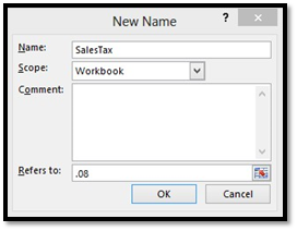
Click OK.
To see all the names you've created (if you need a reminder), click the Names Manager in the Defined Names group.
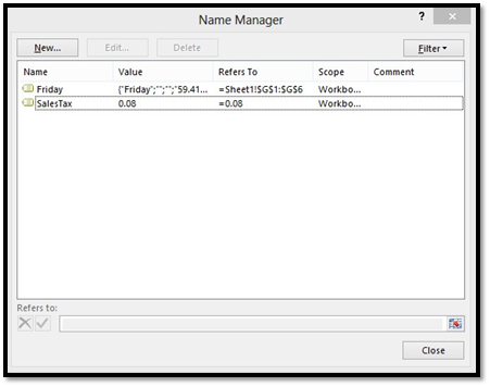
In the dialog box above, you can add, edit, or delete names.
Now, let's go back to the SalesTax name for a minute. We now have a reference for sales tax. We can then use that reference in a formula. In the example below, we'll apply sales tax to the total for Friday, which is cell G8.
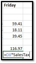
Hit Enter.
We now get the amount of sales tax.
We can now add (SUM) the amounts from G8 and G9 together to get a grand total.
There are two kinds of cell references; Absolute and Relative.
A relative reference in a formula depends upon its position in a worksheet. For instance, the cell coordinates in the following example -- "B4:B6"-- are relative references.
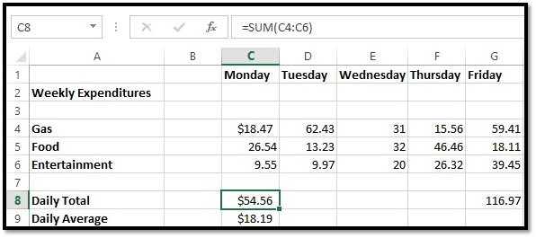
In the example below, we can copy the formula in cell C8 and paste it as a formula into cell H8 (not shown in the snapshot below).

When we do this, the formula stays the same, but the relative references change.
Let's look at the formula bar to confirm that the formula is the same, but the references changed:
This is because MS Excel recognizes the relationship between the formula in cell B7 and its cell range (C4:C6). When we paste the formula into a new cell, it creates the same relationship in the new position.
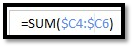
An Absolute Reference does not depend upon its position in a worksheet. For instance, if the value in cell C8 were an absolute reference, when we pasted the formula in cell H8, the formula would read: =SUM($C$4:$C$6).
The symbol "$" in cell coordinates tells MS Excel that this is an absolute reference. To create an absolute reference, type a dollar sign before the column reference in the formula. You can also type it before a row or both.
A Mixed Reference contains both an absolute reference and a relative reference. Which means, it can either contain an absolute column and a relative row, or a relative column and an absolute row.
At some point when using Excel, you may want to copy a formula, then paste it into a different cell. You may want to keep the formula and the values the same in the formula.
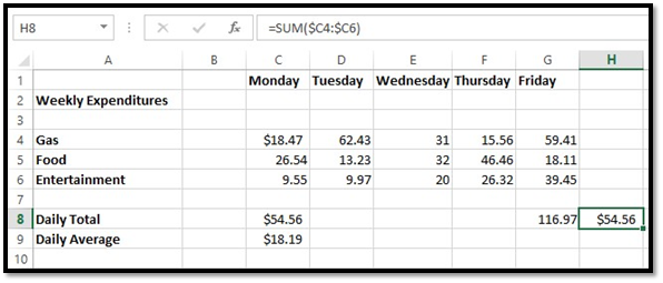
In the snapshot below, we want to copy the formula and the values from cell C8 and paste them into H8 (not shown in the snapshot).
Let's learn how to do it.
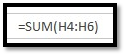
As you can see, C8 contains relative references. This means when we copy, then paste the formula to cell H8, Excel will change the cell references to match the coordinates. Instead of the formula being =SUM(C4:C6) it will become =SUM(H4:H6).
Let's change it to absolute references.
We don't want the references to column C to change.
Now, we can click on cell C8. You can either click Copy under the Home tab in the Clipboard group, of you can right click and select Copy.
Now click on the cell that you want to paste into. For us, it's H8.
Right click and select Paste Special.
We want to paste the formula.
Click OK.
As you can see, our formula, with our absolute values, appears in cell H8.
If you don't add absolute values to your formula in the cut/copied cell, it will change the cell references to the pasted cells coordinates, as mentioned above.
You can also simply paste the calculation and value from a formula in one cell into another.
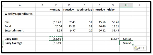
Copy cell C8. This time we'll paste into H9.
Go to cell H9 and right click, then choose Paste Special.
In the Paste Special dialog box, check Values, then click OK.
As you can see in the snapshot below, the value was pasted. If you look in the Formula Bar, you'll see the formula wasn't pasted.
Linking Formulas
When you paste a formula, you may want to link back to the cell where you copied the formula. There may be data there that needs referenced, etc.
To link formulas, first select the cell that contains the formula that you want to copy.
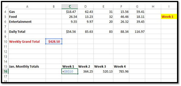
We've chosen C10.
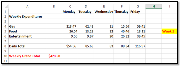
We want to move B10 down further on our worksheet where we do monthly totals, but we want to link to the week shown above.
Here's the monthly total section of our worksheet:
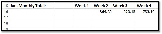
We need to fill in Week 1 in cell C16 with the calculation from cell B10.
First, we need to copy B10.
Next, we go to C16 and choose Paste Special.
Click the Paste Link button at the bottom left side of the window.
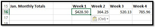
As you can see, the calculation is now pasted into the cell above.
Now, if you look at the Formula Bar whenever you click on cell C16, you'll see it links you to cell B10.
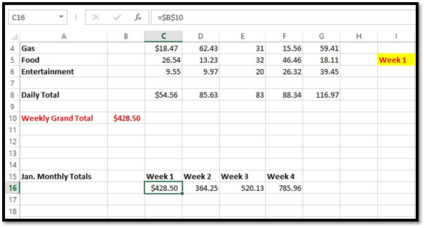
If you double-click on C16, you'll see the original formula appear in cell C16 (notice the references were changed to absolute by Excel), and cell B10 is highlighted in blue.