Whenever you save an Excel file to your computer, or save it using any other method, it's saved as a workbook. A workbook is made up of worksheets. In other words, worksheets are stored in workbooks, and workbooks are the files that you actually save.
Opening Worksheets and Workbooks

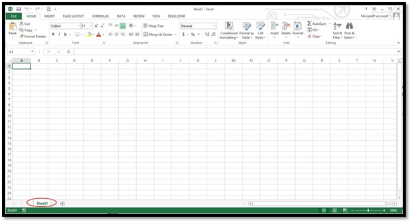
When you open a workbook, you see the worksheets. If there's more than one worksheet in a workbook, all worksheets will be marked by sheet tabs at the bottom of the worksheet area.
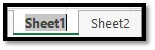
The sheet tab is circled in red below:
Individual worksheets within the workbook may be opened by clicking on the Sheet Tabs at the bottom of the spreadsheet screen.
Opening an Existing Workbook
If you want to open an existing workbook, you can do one of two things. You can find the file on your computer, then double click to open it.
However, if you already have Excel open, you can go to the Backstage area by clicking the File tab. Click Open on the left.
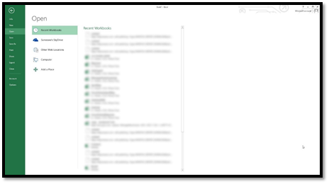
You can then search through recent workbooks, your SkyDrive, other locations on the web, your computer, or you can also add a place you want Excel to look.
About Sheet Tabs
You can add or subtract worksheets, as you'll learn later. For now, it's important to know how to access the sheets.
In the picture above, Sheet 1 is in white, with green writing. Click on the tab to open the sheet.
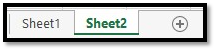
If there is more than one sheet, as shown below, we'd click on the tab that represents the sheet we want to open.
Remember, each sheet tab represents a worksheet in the workbook.
The default names that MS Excel 2013 assigns worksheets are Sheet 1, Sheet 2, Sheet 3, etc. However, as you use Excel to create your own spreadsheets, you'll want to assign different names so you know which spreadsheets contain what information.
Let's rename Sheet 1 for this example.
The easiest way to rename a sheet is to move the arrow over the sheet you want to rename, then right click on it with your mouse.
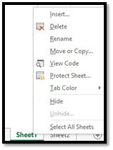
Select Rename.
When you do this, Sheet 1 will be highlighted (selected). You can type in the new name.
Now simply type the new name. When you're finished, click in the worksheet area.
To add a worksheet, go to the Sheet Tabs. Click the plus sign (+) that's to the right of the last worksheet, as shown below.
Here are some things to remember when adding worksheets:
-
Click the sheet tab that will come before your new sheet tab/worksheet.
-
For example, if you want to put a new worksheet/sheet tab after Worksheet 2, click Sheet 2, then click the plus sign.
Excel then adds the new worksheet and gives it the default name. You can then change the name.
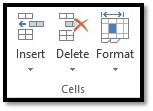
Note: You can also go to the Home tab on the ribbon. Go to the Cells group and click Insert, then select Insert Sheet.
To delete a worksheet, go to the Sheet Tabs, select the worksheet that you want to delete, right click, and select Delete.
Hiding a worksheet allows you to remove it from view of others or simply get it out of your way. When you hide a worksheet, you or anyone else accessing the file will not be able to see it. There will not be a Sheet Tab for it. You'll have to unhide it to be able to view it again.
First, select the worksheet you want to hide by clicking on its tab.
Next, click on the Home tab and go to the Cells group. Click Format.
Select Hide and Unhide from the Visibility group in the drop-down menu, then Hide Sheet.
To unhide a worksheet so that you may view it again, follow the same steps as you took to hide the worksheet, except this time select Unhide Sheet.
You can also hide data by hiding cells, rows, and columns within a worksheet. There are a few reasons you may choose to do this. It may be to simplify the worksheet and make it easier to navigate or to protect certain information.
As with all Microsoft products, there is more than one way to do a certain task. You can use the steps above for hiding sheets to hide columns and rows. But there's also another way. Let's learn how to hide columns by using the Column Header Bar. This is the bar where the column letters are: A, B, C, etc.
Remember, when you hide a column, data in that column can still be used in the worksheet.
To hide a column:
Right click on the column header of the column that you want hidden. We're going to use column A in this example.
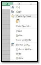
When you right click on the column, the entire column will be select, and a menu box will appear. Select Hide from that menu box. This will hide the column.
To unhide the column, follow the exact same steps and, instead, select Unhide.
Let's say, for example, that we want to hide columns A, B, and C. The first thing we're going to do is left click the mouse on the column A header. This selects column A. Keeping the left mouse button pressed in, we're going to drag it over columns B and C to select them as well. See the screen shot below.
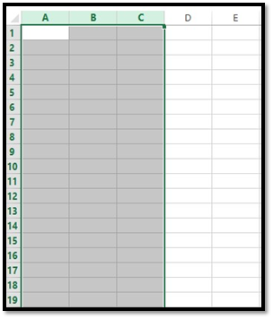
When the columns are highlighted, right click the mouse and select Hide. This will hide all three columns.
If you want to hide more than one column, but the columns aren't adjacent, there's an easy way to do it. Simply click on the first column to be hidden. Press and hold down the Ctrl key on your keyboard while you left click on the other columns to be hidden. Now, right click on one of the columns that you selected and choose Hide from the menu. This will hide all the selected columns.
You can easily hide rows in MS Excel 2013 in the exact same way that you hide columns. The only difference is that you're going to click on the number of the row that you want to hide. In the snapshot below, we clicked on row 1. This selected (highlighted) the entire row. Next, right click your mouse and select Hide.
When you enter any sort of data into Excel, you'll enter it into a spreadsheet. Of course, starting to enter information is as simple as clicking on a cell in the spreadsheet and typing, but there are some things that are helpful to know � and that you can do � before you ever type that first letter or number.
The first thing you want to do before you type anything, is to spend a little time planning the spreadsheet. Beginning to type in Excel is perhaps not as easy as it might be in a word processing program, because you're going to enter all information into rows and columns. A little more organization is required to save you the time of having to create, and then recreate, the spreadsheet to get it as you want it.
To organize your spreadsheet, you'll need to determine:
-
What is the point of the spreadsheet?
-
What information do you need to include?
-
What headings are you going to need to explain the information in the spreadsheet?
-
Do you want to use columns, rows, or both?
Take a little time to plan out your spreadsheet, and you'll save yourself a lot of time and headaches down the road.
There are three types of data in Excel: text, value, or formula. This is the type of data you enter into cells.
If Excel detects the entry is a formula, it will calculate the formula and display the result in the cell. You can see the formula in the Formula Bar when the cell is active.
If it detects that it's not a formula, Excel then decides if it's text or value.
Text entries are aligned to the left side of the cell.
Values are aligned to the right.
This is all important to know so you can make sure you are entering things correctly, and Excel is recognizing them for the type of data you are trying to enter.
Text entries are simply bits of data that Excel can't classify as a formula or value. Most text entries are labels � or the names of columns and rows.
You can always tell if Excel is classifying your entry as text because it will be aligned to the left side of the cell.
Values are the building blocks of all formulas that you enter. Values are numbers that represent quantities, and they are numbers that represent dates.
Values are aligned to the right side of the cell.
If Excel cannot solve the values you add as a formula, it will assume they are values.
If you need to add a negative value, enter a minus (-) sign before the value. You can also put it in parentheses if you want. Excel will convert it to a negative if you choose to do it that way.
If you're entering a value that's a dollar amount, you can add dollar signs and commas just like you would if you were handwriting it.
If you need to add a decimal point, use the period key on your keyboard.
If you need to convert a fraction to a decimal, Excel can do that for you, so there's no need to stress over it yourself.
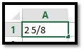
Simply type the fraction in using the slash key on the keyboard. Just make sure you leave a space after any whole numbers before typing in the fraction, as shown below.
Hit Enter.
As you can see, Excel classified the number as a value and aligned it to the right. However, it's still a fraction.
Now look at the Formula Bar (make sure the cell is active first):

Excel converted it to a decimal.
Note: If you're entering simple fractions such as 5/8 (where a whole number isn't present), you must enter a zero as the whole number. If you don't, Excel thinks you're entering a date.
For now, however, it's important that you get a feel for formulas, what they are, and how they work.
In Excel, a formula is simply an equation that performs a calculation. It can be as simple as 5 + 2, or as complex as  . You can perform calculations within a single cell or based on the values in two different cells, a range of cells, or even a range of cells across several different worksheets.
A formula must start with an equals sign: =. This might seem strange at first since ordinarily an equals sign comes at the end of an equation, but this lets Excel know right away that you want to perform a calculation. Whenever you want to add a formula in Excel, you always start with the equal sign, as shown below:
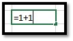
The snapshot above shows a very simple formula.
Once you've entered it into the cell, either hit Enter or the arrow key to go to another cell.
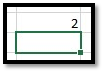
Excel performs the calculation and displays the answer in the cell.
However, whenever you click on the cell, the formula will appear in the Formula Bar:

If you need to enter a bunch of numbers that use the exact same number of decimal places, you can use Excel's Fixed Decimal setting so that Excel automatically adds the decimal point for you.
To do this, click the File tab to go to the Backstage area, then click Options on the left.
Click Advanced on the left.
Go to Automatically Insert a Decimal Point and put a check in the box.
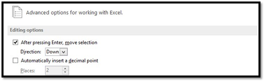
By default, it's set to two places from the left. You can change this number.
Dates and times are values in a worksheet, not text, because they can be used for formulations, such as how many days an employee worked last month. In saying that, Excel determines that you're entering a date or time by the way you type it in.
These are the ways you can type a time into Excel so that it recognizes it as a value:
-
5 AM or 5 PM
-
5 A or 5 P
-
5:46 AM or 5:46 PM
-
5:46:12 AM or 5:46:12 PM
-
17:46
-
17:46:12
Below are the date formats that Excel recognizes as values:
-
May 1, 2013 or May 1, 13. It will appear in Excel as 1-May-13
-
5/1/13 or 5-1-13. It will appear as 5/1/2013
-
1-May-13 or 1/May/13 or 1May13. It will appear as 1-May-2013.
-
May-1 or May/1 or May1 will appear as 1-May.
Note: You only need to enter the last two digits of the year for this century if the last two digits are 00-29. Starting with 2030, you need to enter all four digits.
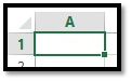
Now that we've covered some of the very basics of data, it's time to start actually entering information into Excel. Entering information is as easy as clicking on a cell. When you click on a cell, the cell will be highlighted with a green border as shown below.
Once it's highlighted with a border, you can type inside of it. When you're finished entering information into one cell, you can click the mouse in another cell to type more information.
However, moving and clicking your mouse each time you want to change cells becomes time-consuming. Most people who use Excel want to move a little faster than that and save as much time as possible. That said, you can also use the following keys to navigate the spreadsheet as you enter information.
-
Enter. Enters the data into the current cell, then moves the cursor to the next cell in the same column. In other words, using the example above, if we pressed 'Enter' it would move the cursor down to cell A2. We could then type in A2.
-
Tab. Tab enters the data into the current cell, then moves one cell over in the same row. In this example, it would move to B1.
-
Arrows. You can navigate through columns or rows in the spreadsheet using the arrows.
-
Esc. Cancels the current entry
Labels are used for things such as titles, headings, names, and for identifying columns that contain data. These are text values.
Below we've created the beginning of a spreadsheet that will be used to calculate the sales for each employee, by the month.
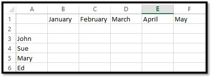
As you can see, Excel recognized our entries as text values. This is correct because what we entered was labels.
Now, let's say we want to add Mary twice in our spreadsheet.
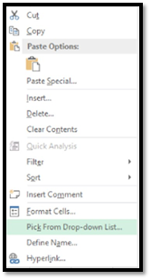
A method that you can use to quickly enter repeated labels is to use the Pick List feature. All you have to do is right click on any cell, then select 'Pick from List.' It will provide a menu of all other entries in cells from that same column. See the snapshot below.
When you click on Pick from Drop-down List, a drop-down box will appear:
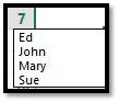
Select the label you want to appear by highlighting it, then clicking the mouse.