Microsoft Excel is a spreadsheet program that comes packaged with the Microsoft Office family of software products. Just like the other programs by Microsoft, Excel can be used for a wide variety of purposes such as creating an address book, grocery lists, tracking expenses, creating invoices and bills, accounting, balancing checkbooks and other financial accounts, as well as any other purpose that requires a spreadsheet or table.
Excel is much more than a basic spreadsheet program. It gives you the complex tools and features you need to design professional spreadsheets, but all with just a few clicks of the mouse.
The good news is that Excel makes everything easy. By learning how to navigate the program, and where to find each feature, operating Excel can become a breeze!
You can use Excel to:
-
Organize, sort, and record data.
-
Enter in text and mathematical data.
-
Keep statistics.
-
Keep records.
-
Create mathematical equations and functions to accurately keep records, statistics, and data.
-
And much more!
With the launch of Office 2013, Microsoft made changes in how they sell their most popular software package. Of course, you can download a free trial by simply going to the Microsoft Office page, picking out what version you want to try, then downloading the software. You don't need a credit card to try the software.
If you want to purchase the software, Microsoft now gives you two choices. As always, you can buy the software -- either online or from most office supply or computer stores. The prices to buy the software vary depending on what version you wish to purchase. There are three versions: Home and Student, Home and Business, and Professional. As with other versions of Office, it's a one time charge and the software is yours to use as long as you wish.
However, with Office 2013 also comes Office 365, which is another method that you can use to buy the Office suite of software. With Office 365, you subscribe to the software instead of just purchasing it like you've done in the past. You can pay for your subscription by the month or year on the Microsoft Office website. The price of your subscription will be determined by the version that you want: Home, Small Business, or Mid-size Business.
Once you purchase a subscription, you'll be able to download Office 2013 on your computer just as you would if you had bought the software in a store. As part of Office 365, you'll also be given multiple licenses, which will give you the ability to install the software on other computers, as well. This is a perk that doesn't come with buying the software in a store. For the Home version, you get up to five licenses (five devices). The Small Business version comes with licenses for up to 25 users. The Midsize Business provides for up to 300 users. There's also an Enterprise version for larger companies that offers unlimited users.
Once you subscribe to Office 365, you'll never have to worry about purchasing a new version of Office ever again. When a new version comes out, your software will be updated for you.
Excel 2013 is arguably the best version yet. It contains the same great features you loved in past versions, which have been fine tuned and improved for better usability. In addition, it contains some great new features that make Excel even more useful and functional than ever before.
Here are the improvements:
-
The new Start Screen makes getting started in Excel easier than ever. You can start a blank spreadsheet, or open a template � and get busy!
-
The new Quick Analysis tool makes it easy to convert data into a chart or table. All it takes is two steps (sometimes even less).
-
Flash Fill finishes your work for you in 2013. When Excel detects a pattern in your data, it enters the rest of the data for you.
-
Don't know what type of chart to use? Chart recommendations now shows you the best chart for your data.
-
Improved slicers can now filter data in tables and query tables.
-
Each workbook now has its own window.
-
New functions
-
Save and share files online � for free!
-
Embed your worksheet data in a web page
-
The new Design and Format tabs make it easier to format charts and tables.
-
View animation in charts
-
And more!
You open Microsoft Excel by clicking on the icon on your desktop (if you have one there) or in the program bar. The icon for Microsoft Excel 2013 looks like this:

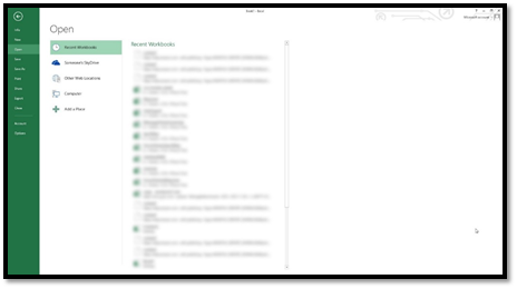
When you click on the icon, Excel 2013 will open, and you'll see the Start Screen. This is new to 2013.
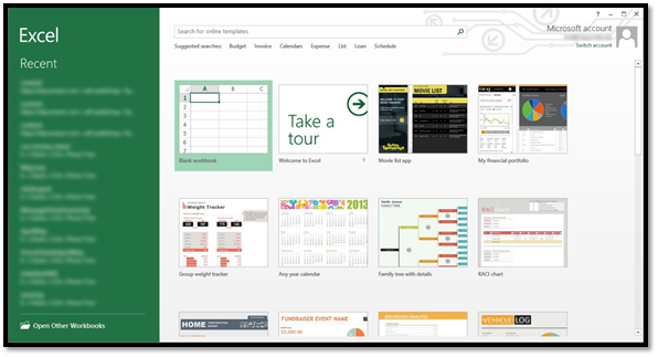
On the left, you'll see the dark green column that contains your recently opened files. You can click on any of these to open them. To the right, you'll see templates you can use to start a new Excel workbook. You can also choose to just open a workbook, as we've selected above.
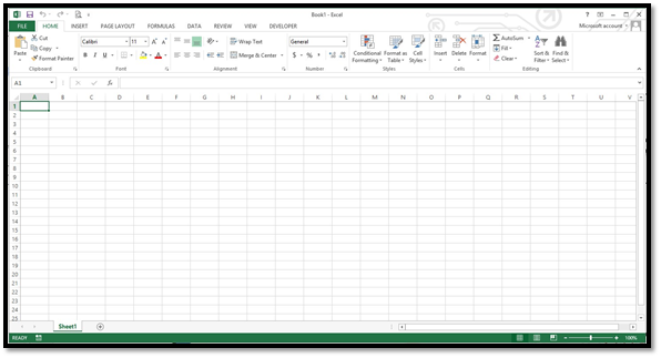
This is a new workbook for which the default name is Book1. You can see the name in the Title bar.

For each additional new workbook that you open, the name increases by one digit: Book2, Book3, etc. If you start MS Excel by clicking on an already existing workbook on your computer, it will open automatically and your workbook will be displayed in the MS Excel window.
Touring the Excel 2013 Interface
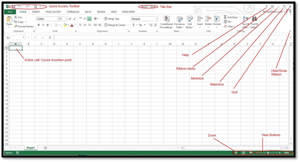
Take a few minutes to look at the features that we've labeled for you. It's not important that you know how to use these things right now. For now, just take a second to familiarize yourself with where everything is located. The items labeled above help to make using Excel 2013 easier, but they're not the bread and butter.

The ribbon is divided into tabs. These tabs are also menus. The tabs are Home, Insert, Page Layout, Formulas, Data, Review, View, and Developer.
Below each tab are commands (or tools) you can use. The commands (or tools) located beneath each tab relate to the tab. For example, under the Page Layout tab, you would find tools to create a page layout.
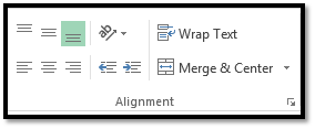
In the Alignment group are all the tools that are related to alignment.
If you look to the right of the word "Alignment," you'll see an arrow in the lower right corner. If you click this, it will take you to the Alignment options dialog box. You can click this arrow in any group to open the options for that group.
If you're using Excel on a tablet, you can adjust the spacing between buttons on the ribbon to make it easier to use. You do this by activating Touch mode.
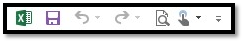
To do this, click or touch the Quick Access Toolbar button:
Select Touch/Mouse Mode.
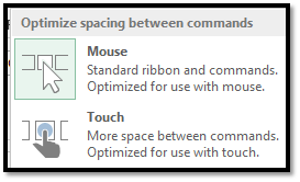
There is now more space between commands on the Ribbon.
Navigating Excel 2013
Learning how to navigate around Excel is critical to being able to successfully use the program. In this section, we're going to focus on the major elements of Excel 2013 and take a few minutes to become familiar with their purpose.
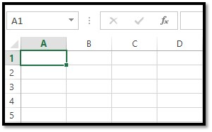
Understanding the Basic Elements of an Excel Spreadsheet
Before going any further in this section, it's important to understand the elements of a spreadsheet, in Excel, or any spreadsheet that you may use.
The cell above is highlighted because it's an active cell. In other words, we clicked on it with our mouse to make it active so we can enter data into it.
Now, all the cells in a worksheet are organized into columns and rows. In Excel, rows are represented by numbers. Columns are represented by letters.
Below is a snapshot of row 5, followed by a snapshot of column C.

Since rows and columns are labeled with numbers and letters respectively, you can also locate the exact coordinates of a cell.
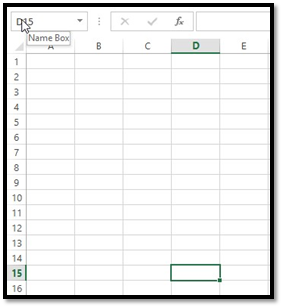
For example, instead of your boss coming to you and telling you the number for March's expenses for employee Susie Smith are wrong, he can simply say, recheck the number in D15. This would tell you to go to column D, row 15.
Enter the coordinates for the cell. We're going to enter D15, then hit Enter.
As you can see below, Excel took us to the exact cell and highlighted it for us.
The Formula Bar
The formula bar is the magical ingredient of the soup, so to speak. It is what makes Excel easier to use than doing spreadsheets by hand, or using other programs where you're left to do the math by yourself.
In this section, you'll learn how to enter formulas and equations into MS Excel 2013. The formulas and equations that you enter will be entered in and displayed in the Formula Bar. It is located to the right of the Name Box.

The Formula Bar has the fx to the left of it.
On the left side of the Formula Bar are the Formula Bar buttons. The Insert Function button is fx. When you start making or editing a cell entry, X is Cancel and the check mark is Enter.
The white area (or bar) to the right of the buttons is the Cell Contents area. The Formula Bar always shows you the contents of a cell, even if it doesn't appear in the cell. In other words, it shows equations in the cell even if the cell only displays the answer to the equation. It will show contents of cells that appear to be blank in the spreadsheet as well. If the Cell Contents area is blank, you know the cell is empty.
Using the Backstage area, you can open an existing spreadsheet, create new spreadsheet (either blank or template), save workbooks and spreadsheets, share workbooks and spreadsheets, print, close, and set options for the Excel program.
Click the left facing arrow at the top left of the Backstage area to go back to your spreadsheet.
You can use the Quick Access toolbar to add shortcuts to tools that you use frequently, rather than having to click tabs and find the tools in a group.
By default, our Quick Access toolbar displays these shortcuts:
 Save
Save
 Undo
Undo
 Redo
Redo
 Print Preview/Print
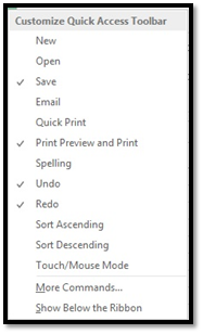
You can customize the Quick Access toolbar and add shortcuts so the tools you need appear there for easy access.
Click the drop-down menu to the right of the toolbar. It looks like this: 
If you want to add a shortcut for a tool, but you don't see it on the Customize Quick Access Toolbar list, you can still add it to your toolbar. You do this by adding Ribbon commands.
Simply go to the Ribbon and find the tool that you want to add. Right click on the tool (or tab and hold if you're using a touchscreen device).
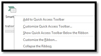
Select Add to Quick Access Toolbar.
As you can see, it's now added:
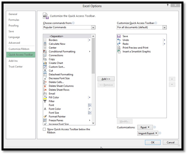
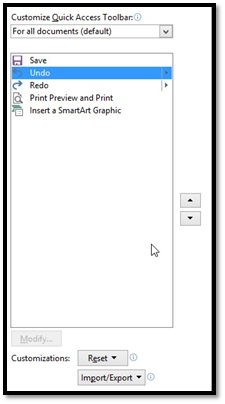
On the right side, you can see everything that's added to the Quick Access toolbar. They are listed in the order they appear on the toolbar.
If you want to group buttons on the Quick Access toolbar, you can add vertical separators. To do this, select <Separator> from the list on the left:
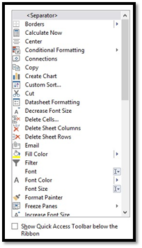
Then click the Add button twice.
To add shortcuts listed in the left column, click the shortcut to select it, then click the Add button.
To remove shortcuts from the Quick Access toolbar, select the shortcut in the right column, then click the Remove button.
Being able to navigate through a worksheet will make using Excel a lot easier. However, before we discuss that, let's quickly review three things you have to know about the worksheet area. Remember, the worksheet area contains cells, rows, and columns.
-
The cell cursor is the dark green border that appears around a cell. It means a cell is active.
-
The location of the cell, or address, appears in the Name box.
-
The cell's row number and column letter are shaded. Look at the snapshot below. Note that the row number 1 is shaded differently than the rows after. Note that the column A is shaded differently than the other columns.
Now, since the Excel worksheet contains so many cells, rows, and columns, not all of your cells are going to be displayed at once on the screen. For that reason, there are several ways that you can use your mouse cursor to move through and navigate your worksheet.
Of course, if the cell is displayed, you can simply click on it to make it active. If you're using a touchscreen, just tap it.
You can also type the coordinates in the Name box and be taken to the cell.
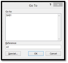
All you have to do is type the address of the cell in the Reference box (pictured above).
You can also use cursor keys to move to the desired cell. The cursor keys are displayed in the table below:
|
Keystroke |
Action |
|
Moves cell to the right |
|
? on the keyboard or Shift+Tab |
Moves cell to the left |
|
Up arrow on the keyboard |
Moves one cell up |
|
Down arrow on the keyboard |
Moves one cell down |
|
Home |
Moves cursor to cell in Column A of the current row |
|
Ctrl+Home |
Moves cursor to the first cell -- A1 |
|
Ctrl+End or End, Home |
Moves the cursor to the cell that's at the intersection of the last column with data and the last row that has data in it |
|
Page Up |
Moves the cursor to cell that's one full screen up in the same column |
|
Page down |
One full screen down (in the same column) |
|
Ctrl+? or End, ? |
Moves the cursor to the first occupied cell that's to the right that's has a blank cell before it or after it. If there isn't an occupied cell, it goes to the end of the row |
|
Ctrl+? or End, ? |
Same as above, except first occupied cell to the left. |
|
Ctrl+ Up arrow, or End, Up Arrow |
Moves the cursor to the first occupied column above that has a blank cell before it or after it. |
|
Ctrl+Down arrow, or End, Down arrow |
Same as above, except for first occupied cell below. |
|
Ctrl+Page Down |
The cursor moves to the next worksheet of the workbook |
|
Ctrl+Page Up |
Moves to the previous sheet of the workbook |
Using the Touch Keyboard
If you're using Excel on a tablet or other touch-enabled device, you can also use the on-screen touch keyboard. Instead of entering characters (letters, numbers, and spaces) by pecking away on your keyboard, you'll simply touch your finger or stylus pen to the keyboard on the screen.
Make sure you enable Touch mode before starting to use Excel from a tablet or touch device.
To use the on-screen keyboard, simply tap in the spreadsheet area to see the cursor � and the keyboard.
The Status Bar appears at the bottom left of your Excel window. It contains the following information about your spreadsheet:
-
Mode Indicator shows the state of your Excel program, such as Ready, Edit, etc. It will also tell you if any special keys are in use, such as Caps Lock.
-
AutoCalculate Indicator shows the average and sum of all the numerical entries for the current cell selected, as well as the count of every cell in the selection.
-
Layout Selector allows you to select between three different layouts for the worksheet area: Normal (default), Page Layout View, and Page Break View. We'll discuss views later in the section.
-
The Zoom Slider lets you zoom in and out of areas on a worksheet to see more/less cells.