Worksheets and Workbooks in Excel 2019

After you become familiar with Excel 2019's basic menus and functionality, it's time to enter data into a worksheet and see the way Excel works with it. When you hear "spreadsheet" in discussions about Excel, you generally think of an Excel file. However, Microsoft makes a distinction between worksheets and workbooks. As you work with multiple Excel files, you'll need to know the difference between the two properties.
Worksheets vs. Workbooks
It might seem like an insignificant distinction, but when you start working with formulas and linked files, understanding the difference between a worksheet and a workbook is important in Excel. When you create a new Excel file, you make a new workbook. A workbook is synonymous with an Excel file.
After you create a workbook, Excel 2019 automatically creates a new sheet. You can see the name of the sheet at the bottom-left of the opened workbook window.
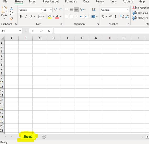
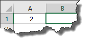
(An Excel workbook with one worksheet)
The default name of the worksheet is "Sheet1" as you can see in the image above. Excel allows you to create several worksheets within one workbook. Each sheet can be used to store data organized by type, and each sheet within the workbook can reference others within the workbook. For instance, you could have two sheets within a workbook named "CustomerOrders." One sheet has customer shipping information and the second sheet has order information. A worksheet with customer orders can reference the worksheet with customer shipping data to determine the address to send product.
Notice the "+" image next to the sheet in the image. Click it and a new sheet is created with the next numerical value in the name. The first sheet's default name is "Sheet1." When you create a new sheet, the next sheet name is "Sheet2." Each worksheet in an Excel 2019 workbook must be given a unique name, even if you keep the default names applied to your worksheets.
You don't have to keep the default name. You can change a worksheet's name. Double-click "Sheet1" on the first worksheet tab and notice that Excel prompts you for a new name. Type any name in the text box, and it's applied to your worksheet. This new name is stored as the worksheet's name. Since you can only have unique worksheet names, you must give each of your worksheets its own name.
Entering Data in a Worksheet
With your worksheet set up, you can enter data in cells. Excel 2019 has several different formatting tools, so this section just describes some basics of entering data and working with alphanumeric values versus calculations and numbers.
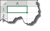
Remember that the "A" label indicates the first column, and "B" is the label for the second column. Since both cells use the row number "1," you know that data should be entered into the first row.
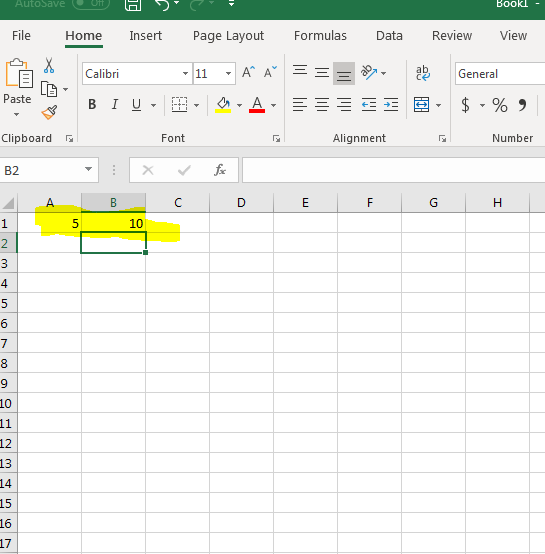
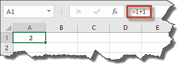
(Data entered into cells A1 and B1)
Now enter the value "001" into cell C1. Notice that Excel 2019 strips the zeros from the value and only displays "1" in the cell. This is because Excel attempts to determine the type of data entered into a cell and formats it appropriately. Unfortunately, Excel doesn't always accurately determine the data type and displays numbers incorrectly. Microsoft provides a way for you to override the default behavior and force Excel to display values exactly how you enter them.
Go back to C1 and change your input from "001" to '001 (notice the single tick mark in front of the first zero). The single tick mark tells Excel to stop determining the data type and only display data exactly how it's entered. Notice that now your spreadsheet displays 001 without Excel removing the zeros. Whenever you enter data that isn't formatting properly, you can always add a single tick character to stop the default formatting.
Sometimes you just want to use a calculation in a cell. This can be convenient when you have several numbers that you can't add without a calculator, so instead you can use Excel's internal calculator to do it for you.
The equal sign ( = ) is the character used to indicate that you want to use a calculation in a cell. One of the main reasons to use Excel 2019 over any other type of software to store data is the ability to use formulas and calculations. You can perform the same actions in any other office software, so Excel is perfect for calculations from basic addition and subtraction to complex formulas using calculus. The hardest part of using Excel for these calculations is knowing how to translate a basic math equation to Excel "language."
For basic calculations, you just need to add the equal sign at the beginning of your data entry. With your spreadsheet open, enter the following data into cell D1:
=4+3
In the above example, we just want to add two numbers 4 and 3. You can calculate any number of values, so you aren't limited to just two numbers.
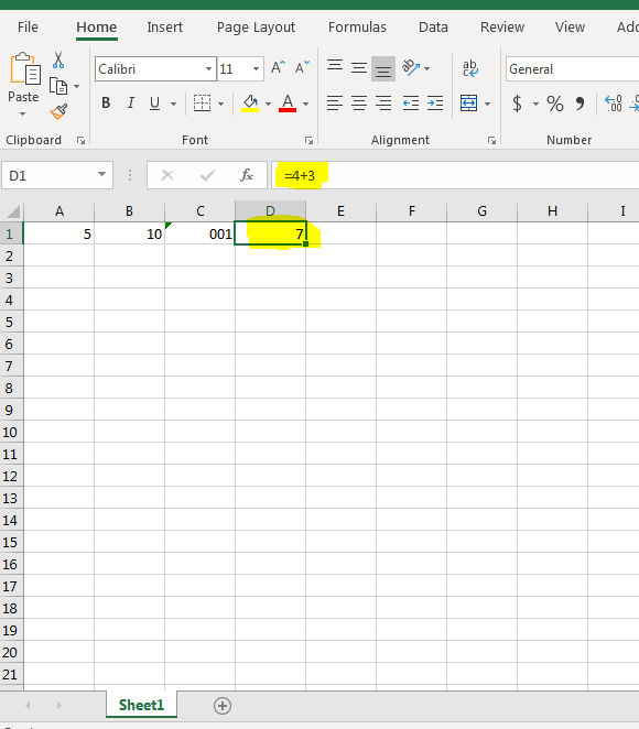
(Cell D1 with a calculation to add two numbers 4 and 3)
In the image above, notice that the value "7" displays although the value entered was "=4+3" in cell D1. When Excel 2019 performs a calculation, it displays the result. Click the cell to see the calculation in the text field located under the menu.
You might make a mistake in your calculation. For instance, you might enter a letter instead of a number in the cell, and Excel picks up on the error. When you have an error in your equation, Excel 2019 displays a message since it can't make a determination how to display results.
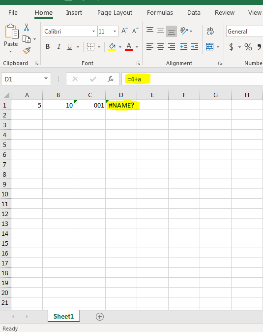
(Displayed text with an error in a math equation)
Notice that instead of a "3" entered, the character "a" was used in the math calculation. Because you can't use a letter in a calculation, Excel doesn't know how to treat it and displays "#NAME?" in the active cell. This display is how you know that there is an error in your calculation.
Referencing Other Cells in Calculations
Excel provides ways to dynamically calculate values in cells based on the values entered into those cells. This is done by entering values in cells and then using one separate cell to display results. Delete all values entered into your current spreadsheet. Re-enter 5 into A1 and 10 into B1, the same values and cells used in the previous example.
Suppose that you want to use the values in A1 and B1 to perform a calculation that you display in C1. You can reference the two values using their A1 and B1 labels. In cell C1, enter the following calculation:
=A1+B1
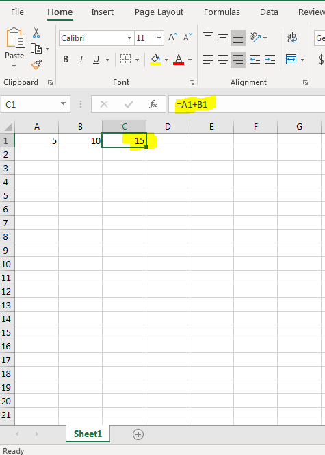
(Calculations using two external cells)
With calculations using cells other than the active one, notice that you still use the equal sign to tell Excel that you want to perform a calculation, but instead of using static numbers, you use the cell name. When you reference cells by name, you can now add new data and the referencing cell will automatically recalculate the results. Using the same spreadsheet, now change the number "5" in A1 to "10."
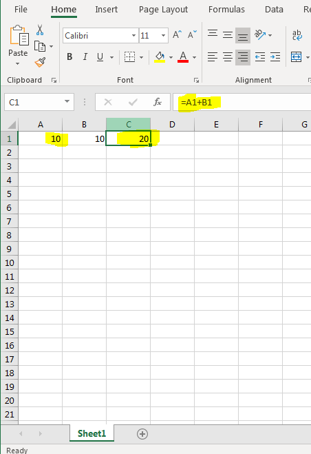
(Changes in entered values are recalculated in C1)
Now that the value "5" was changed to "10," Excel detects the change and recalculates the equation. In this example, the value 20 is now shown in cell C1. Notice that no changes were made to the text entered into C1. It still remains the same, and still references the same cell labels. However, now the value displayed is updated to the latest calculations. What's convenient about Excel 2019 is that this action is done automatically. You don't need to click any buttons or manually update results. Enter new values into your spreadsheet, and all of your formulas and equations update dynamically.
Dynamic updates and re-calculations have several benefits. For instance, suppose that you need to keep track of your expenses each month. To find out what you spend on utilities, groceries and gas, you need to have three different calculations. You can create an Excel spreadsheet with three cells that reference data in three other cells. As you enter different data each month, the calculations will be performed automatically as you enter new values.
Suppose that you have several cells that you want to use in your calculation and typing them could lead to typos. You can use your mouse to click each cell to include in your calculation. Using the same spreadsheet, enter the number "5" in cell F1. Then click C1, which is the cell that displays results of your calculation.
Add the plus character to the equation and then click F1 with your mouse. Notice that Excel automatically adds the cell label F1 to your calculation.
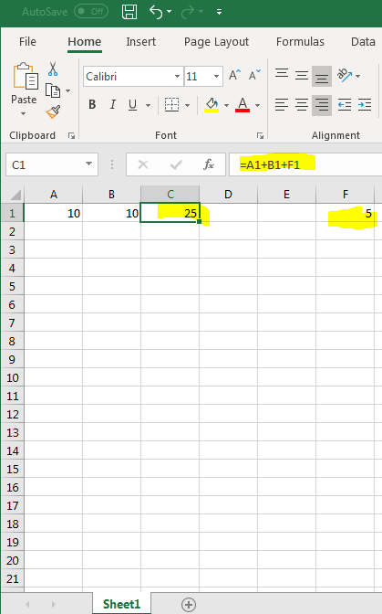
(A third cell added to an Excel calculation)
You can add several cells at a time in your calculation using the mouse. Add another plus character to the active cell and hold the CTRL keyboard key. Use your mouse button to highlight all cells that you want to use in the calculation.
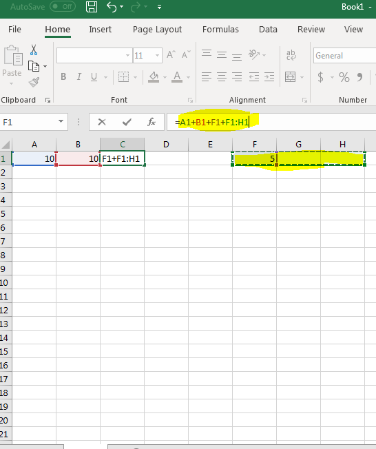
(Multiple cells added to a calculation)
Notice that Excel uses the colon character to indicate a range of cells. In this example, the range F1 to H1 are added to the calculation. Any values entered into these cells will be added to the result. If no values are entered into these cells, Excel treats them as zero and no changes are made to results.
As you work with more data in Excel, you'll use more formulas and calculations. They can then be used in your charts and graphs. Using the mouse, adding multiple cells at once to a calculation takes only a few seconds rather than typing each cell individually. Use these basic techniques to create simple spreadsheets that track your data.
The Three Types of Data
There are three types of data in Excel 2019: text, value, or formula. This is the type of data you enter into cells. If Excel detects that the entry is a formula, it will calculate the formula and display the result in the cell. You can see the formula in the Formula Bar when the cell is active.
If it detects that it's not a formula, Excel then decides if it's text or value. Text entries are aligned to the left side of the cell. Values are aligned to the right.
This is all important to know so you can make sure you are entering things correctly, and Excel 2019 is recognizing your entries as the correct data type.
About Text Data
Text entries are simply bits of data that Excel can't classify as a formula or value. Most text entries are labels. Labels are the names of columns and rows.
You can always tell if Excel is classifying your entry as text because text will be aligned to the left side of the cell.
About Values
Values are the building blocks of all formulas that you enter. Values are numbers that represent quantities, and they are numbers that represent dates.
Values are aligned to the right side of the cell.
If Excel cannot solve the values you add as a formula, it will assume they are values.
Adding Values
Let's take a look at how to enter values into an Excel worksheet.
Negative values. If you need to add a negative value, enter a minus (-) sign before the value. You can also put in parentheses if you want. Excel will convert it to negative if you choose to use parentheses.
Dollar amounts. If you're entering a value that's a dollar amount, you can add dollar signs and commas just like you would if you were writing it by hand.
Decimal points. If you need to add a decimal point, use the period key on your keyboard.
Fractions. If you need to convert a fraction to a decimal, Excel can do that for you, so there's no need to stress over it yourself. Simply type the fraction in using the slash key on the keyboard. Just make sure you leave a space after any whole numbers before typing in the fraction, as shown below.
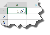
Hit Enter on your keyboard.
As you can see below, Excel classified the number as a value and aligned it to the right. However, it's still a fraction.
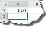
Click on the cell that contains the fraction, then take look at the Formula Bar.
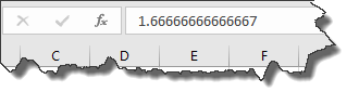
Excel converted it to a decimal.
Note: If you're entering simple fractions such as 5/8 where a whole number isn't present, you must enter a zero as the whole number. If you don't, Excel 2019 thinks you're entering a date.
About Formulas
In Excel, a formula is simply an equation that performs a calculation. It can be as simple as 5 + 2, or as complex as . You can perform calculations within a single cell or based on the values in two different cells, a range of cells, or even a range of cells across several different worksheets. A range of cells is defined as a block or group of cells that have been selected. If all this is confusing right now, don't worry. It will become crystal clear very soon.
For now, remember that whenever you enter a formula into Excel 2019, the formula must start with an equals sign: =. This might seem strange at first since ordinarily an equals sign comes at the end of an equation, but this lets Excel know right away that you want to perform a calculation. Again, whenever you want to add a formula in Excel, you always start with the equal sign, as shown below:
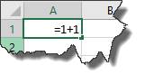
Once you've entered it into the cell, either hit Enter or the arrow key to go to another cell.
Excel performs the calculation and displays the answer in the cell.
Now whenever you click on the cell, the formula will appear in the Formula Bar.
Fixing Decimal Points
If you need to enter a bunch of numbers that use the exact same number of decimal places, you can use Excel's Fixed Decimal setting so that Excel automatically adds the decimal point for you.
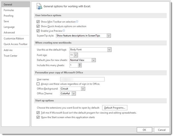
To do this, click the File tab to go to the Backstage area, then click Options.
Go to the column on the left, and click Advanced.
Go to Automatically Insert a Decimal Point and put a check in the box.
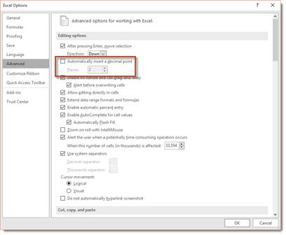
By default, it's set to two places from the right. You can change this number if needed.
Entering Dates
Dates and times are values in a worksheet, not text. They are values because they can be used for formulations, such as how many days an employee worked last month. In saying that, Excel 2019 determines that you're entering a date or time by the way you type it in.
These are the ways you can type a time into Excel so that it recognizes it as a value:
-
5 AM or 5 PM
-
5 A or 5 P
-
5:46 AM or 5:46 PM
-
5:46:12 AM or 5:46:12 PM
-
17:46
-
17:46:12
Below are the date formats that Excel 2019 recognizes as values:
-
May 1, 2019 or May 1, 19. It will appear in Excel as 1-May-19
-
5/1/19 or 5-1-19. It will appear as 5/1/2019
-
1-May-19 or 1/May/19 or 1May19. It will appear as 1-May-2019.
-
May-1 or May/1 or May1 will appear as 1-May.
Note: You only need to enter the last two digits of the year for this century if the last two digits are 00-29. Starting with 2030, you need to enter all four digits.
Entering Data into a Worksheet
Now that we've covered some of the very basics of data, it's time to start actually entering information into Excel. Entering information is as easy as clicking on a cell. When you click on a cell, the cell will be highlighted with a border as shown below.
Once it's highlighted with border, you can type inside of it. When you're finished entering information into one cell, you can click the mouse in another cell to type more information.
However, moving and clicking your mouse each time you want to change cells becomes time consuming. Most people who use Excel 2019 want to move a little faster than that and save as much time as possible. That said, you can also use the following keys to navigate the spreadsheet as you enter information.
-
Enter. Enters the data into the current cell, then moves the cursor to the next cell in the same column. In other words, using the example above, if we pressed ‘Enter' it would move the cursor down to cell A2. We could then type in A2.
-
Tab. Tab enters the data into the current cell, then moves one cell over in the same row. In this example, it would move to B1.
-
Arrows. You can navigate through columns or rows in the spreadsheet using the arrows.
-
Esc. Cancels the current entry
Entering Labels for Columns and Rows
Labels are used for things such as titles, headings, names, and for identifying columns that contain data. These are text values.
Below we've created the beginning of a spreadsheet that will be used to calculate the sales for each employee by the month.
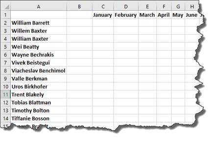
As you can see, Excel recognized our entries as text values. Text values are always aligned to the left side of the cell.
Entering Repeated Labels
Now, let's say we want to add the first name, William Barrett, twice in our spreadsheet.
A method that you can use to quickly enter repeated labels is to use the Pick List feature. To use the Pick List feature, right click on the cell where you want the label to appear. Select ‘Pick from Drop-down List.'
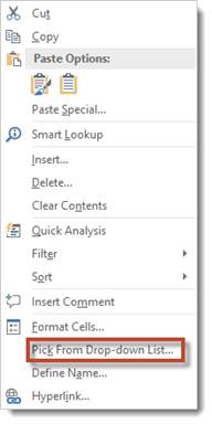
When you click on Pick from Drop-down List, a dropdown menu will appear:
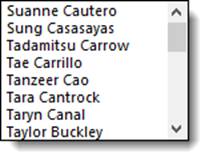
Select the label you want to appear by clicking on it.
For our example, we would scroll down until we found William Barrett, then we'd click on the name. The text label William Barrett is now entered in the cell.