. There is another kind of worksheet that you can create, however. This is called a data list or a database table. These types of worksheets aren't used to calculate values, but to store information, such as names and addresses of clients, or perhaps a library of books.
A data list contains column headings, but no row headings, as you'll see.
Let's set up a new data list and learn how to work with it.
To set up a new data list, click the blank cell where you want to start your list.
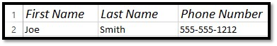
Enter your column headings. These are known as field names.
Next, enter your first row of data below your field names. This is the first record of the data list.
Now, click the Format as Table button in the Styles group under the Home tab. Choose a table style.
Excel puts a marquee around your data and shows you a dialog box that gives the address for the cell range in the marquee. You can edit this if you need to.
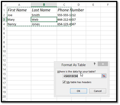
Click OK.
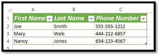
Excel creates your new data list for you.
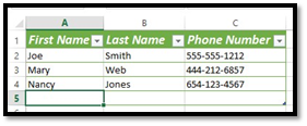
The easiest way to add records to your list is go to the last cell that has data and push the Tab key.
You add rows to lists the same way that you do in a worksheet. Select the row BELOW where you want the new row to appear. Right click and select Insert.
To insert a new column, select the column AFTER where you want the new column to appear. Right click and select Insert.
Any column in your list can be easily sorted by clicking on the downward arrow beside the column heading, as we did below.
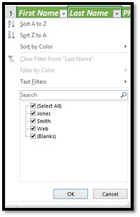
You can sort from A to Z, from Z to A, or by color, and do a custom sort.
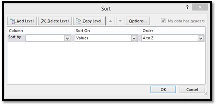
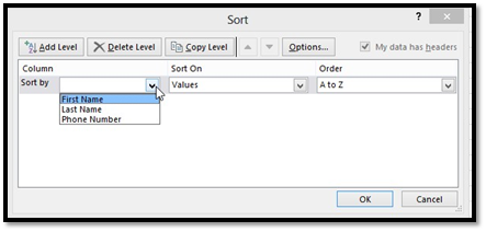
In the Sort By field, choose what you want to sort by:
In the Sort On field, choose what you want to sort on, such as values, colors, etc.
Then select the sort order.
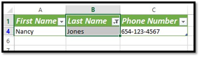
Filtering data in your list is as easily as sorting it. Simply click on the AutoFilter arrow and select the data by which to filter the list.
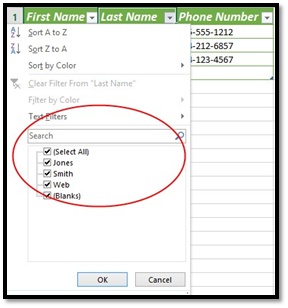
We've chosen to filter the data by the name Jones.
Only Nancy Jones' information is showing. The rest has been filtered out.
Entering and managing lots of data can be a daunting task. It's easy to get overwhelmed in all of those rows and columns of information. The solution is to use a form. A form is simply a dialog box that lets you display or enter information, one record (or row) at a time. It can also make the information more visually appealing and easier to understand.
Most people who are familiar with the MS Office suite associate complex forms with Excel's sister program Access, but you can use them in Excel, as well. In fact, you can even share data between the two programs.
There are two kinds of forms available in MS Excel: data forms and worksheet forms.
-
Data forms are generally used for data entry. They are simple forms that list the contents of a single column. What's more, they can display up to 32 fields at a time. This is especially helpful when dealing with a data range that reaches across more columns than will fit on a screen. You can insert, alter, delete, and even find records with data forms.
-
Worksheet forms are more sophisticated and specialized. They can be customized to fit the information at hand or to fill a particular need. They can even be complex and appealing enough to be printed or distributed online. Worksheet forms must be created using the Microsoft Visual Basic Editor, which is beyond the scope of this article.
The Form button is not included in the ribbon, but you can add it to the Quick Access Toolbar, which, if you remember, is in the upper left corner of the application window.
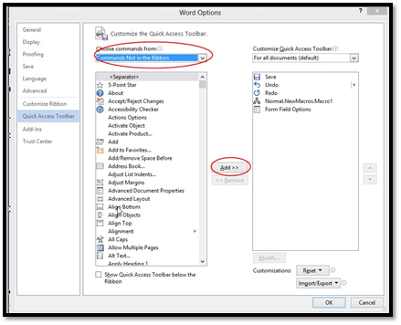
To add the Form button, click the arrow to the right of the Quick Launch toolbar and select More Commands. This will launch the Excel Options window, which can also be accessed by clicking Options on the File tab.
In the "Choose commands from" box, select Commands Not In the Ribbon, then scroll down through the list until you find Forms. Select it and click Add. When you are finished, click OK.
This is what the Form button looks like: .
.
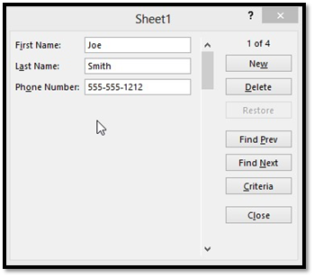
When you click the Form button for the first time, Excel will analyze the row of field names and entries for the first record. It uses that information to create a data form.
Let's click on the Form button now.
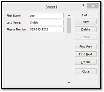
The first record appears in the dialog box:
Click Find Next to find the next record.
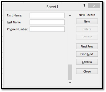
If you want to add a new record using the data form, click New.
As you can see in the snapshots above, the number of the record appears above the New button.
However, when you click the New button, it lets you know that it's a new record.
Let's add a new record.
Enter the information, then hit Enter.
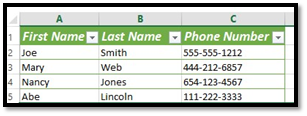
The new record appears in your list:
You can hit ESC when you're done adding records.
In addition to adding records, you can also edit them. You can use the data form to find records that need to be updated or removed from the list.
To do this, click the Form button on the Quick Access Toolbar.
Find the record that you want to update or remove.
Now click in any of the fields to update the data. You can also delete data in the field.
Hit Enter.
If you have a lot of records, navigating through them can be a challenge. The data form makes it a bit easier.
If you want to move to the next record in the data form, press Enter or the down arrow key.
To move to the previous record, hit the up arrow, or press Shift+Enter.
To move to the first record in the data list, press CTRL+ the up arrow, or press CTRL+PgUp.
To go to a new data form that comes after the last record, press CTRL+ down arrow, or CTRL+PgDn.
If you want to find a specific record, you can use the Criteria button in the data form. It's pictured below.
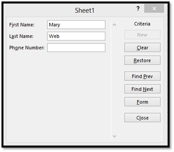
When you click the Criteria button, Excel clears the field entries in the data form. Instead, the word Criteria is displayed.
Let's push the Criteria button to show you what we mean.
We now see a blank data form.
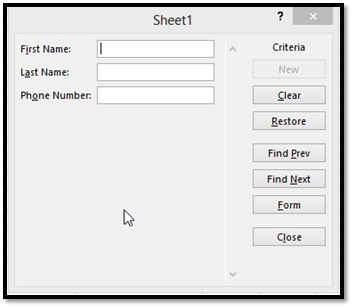
Notice that the word Criteria is above the new button, and the new button is inactive, since we're searching for a record.
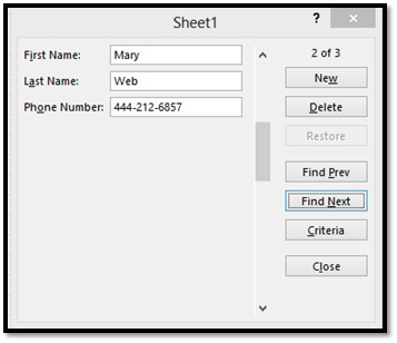
Now, let's say you're looking for a woman named Mary Web, but you have 5000 women named Mary in your list.
Enter the criteria: Mary Web.
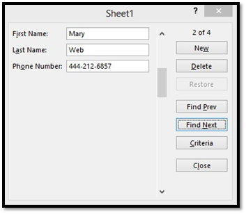
Now click the Find Next button.
As you can see, it brings up the record.
You can also include the following operators in search criteria to help you find the record you need:
? for single
*for multiple wildcard characters
= Equal to
>Greater than
<Less than
<=Greater than or equal to
<=Less than or equal to
<>Not equal to
Data Validation lets you choose what information is acceptable to enter into a cell. For instance, you may have a product code that has four digits. You can set up a cell so that anything other than a four-digit number will display an error message.
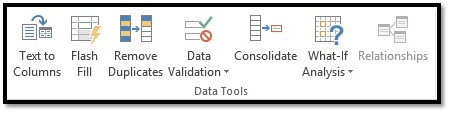
To set up data validation, select a cell or cells, then click the Data tab. Go to Data Validation in the Data Tools group.
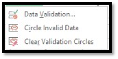
Choose Data Validation from the drop-down menu.
You'll see this window:
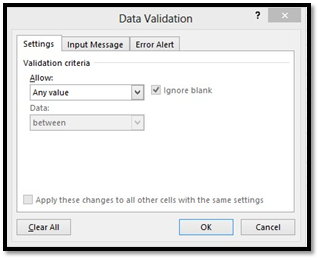
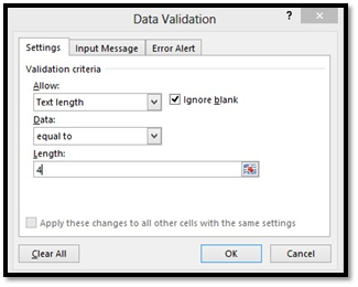
Since we're going to set up a cell to accept only a four-digit number, we will select Text length from the drop-down menu that says "Allow" over it. From the Data drop-down menu, we are going to select "equal to," and in the length text field, we will type "4." That tells Excel we want an entry with four characters.
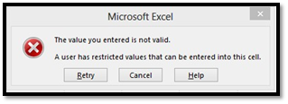
From here, we can hit OK and have Excel provide a generic warning that looks like this:
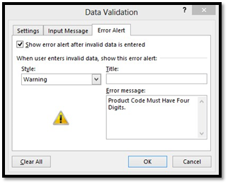
Alternatively, we can create a custom warning by selecting the Error Alert tab, which looks like this:
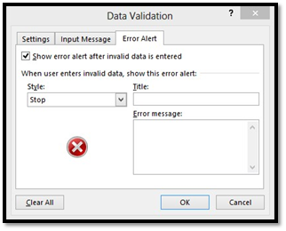
Here we have selected the Warning style and entered the text for our error alert.
When a user enters a code of less or greater than four digits, the message will look like this:
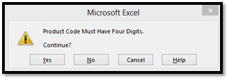
There are three kinds of error messages available in Excel: information messages, warning messages, and stop messages. Information messages and warning messages do not prevent invalid information from being entered into the cell; they simply inform the user that such an entry has been made. Users can choose to ignore the warning. A stop message, on the other hand, will not allow an invalid entry. It has two buttons, Cancel and Retry. Cancel restores the cell to its original value, and retry returns them to the cell for further editing.
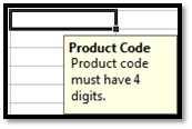
You can also set up a message to remind users what the restrictions or expectations are. Use the Input Message tab to create a custom reminder. It will display anytime the cell, or the range of cells, is selected, as in the example below:
MS Excel 2013 gives you a variety of tools to audit information in a worksheet. Just like data forms, formula auditing can take some of the confusion and frustration out of dealing with lots of different formulas. You can also see which cells have invalid information in them.
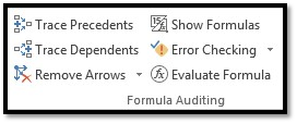
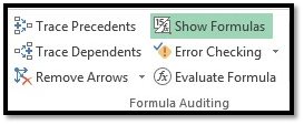
To use these tools, go to the Formulas tab, then the Formula Auditing group.
Select Error Checking and choose Error Checking from the drop-down menu.
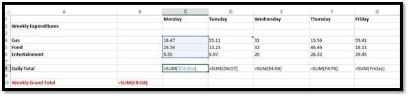
That said, it is not always apparent which cells have formulas in them. Therefore, the first step to evaluate the formulas is to find them. Click the Show Formulas button, as highlighted below.
As you can see in the example below, the whole numbers will be changed to the formulas, and the formula cells will be selected.
To make it easier to see the cells when they are no longer selected, you can click the fill  button. This will fill the selected cells with very visible yellow.
Let's take a closer look at the other functions in the Formula Auditing group.
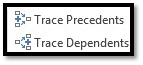
These two buttons allow you to trace (and turn off trace) precedents in a formula. A precedent cell is one that is referred to by a formula in another cell.

B9 through F9 are precedents, because they are referred to in the formula in cell G9. As you can see, the trace precedents button shows you the relationship between the cells.
The next button removes all arrows. 
The Watch Window (pictured below) is useful when you're not sure if alterations to the value in a cell will affect a formula. You can easily remind yourself of the formula by adding it to the watch window.

The Evaluate Formula function will perform the calculations of a formula in slow motion so you can see each step. To use it, select a formula, then click the Evaluate Formula  button in the toolbar. You will see a box that looks like this:
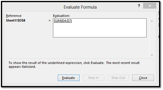
Click the Evaluate button to see Excel perform the calculations in slow motion. Use the Step In and Step Out buttons to navigate through each step in the formula.