Conditional formatting is another way to visualize your data. For example, you can color code cells based on their value.   In this article, we are going to learn more about conditional formatting.

The Highlight Cells Rules

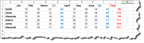
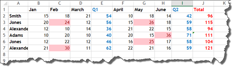
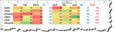
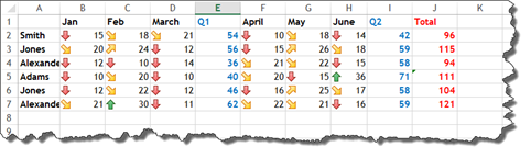
Take a look at our worksheet below.   We want to apply conditional formatting to this worksheet by color coding cells to find out who is selling more than the required quota.   While we could just look at the data to find that out, it is much easier to use color coding to highlight the data.   That makes finding it much easier.

To do this, we are going to select our data.

Next, we go to the Home tab and click the Conditional Formatting dropdown arrow.

Select Highlight Cells Rules.

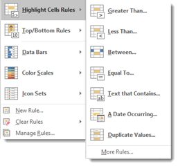
Select if the conditional formatting rule you want to apply will require that the data be greater than, less than, between, or equal to.   Notice that you can also apply highlighting by finding text, dates, or you can even highlight duplicate values in your worksheet.

We are going to choose Greater Than.

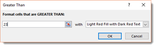
Next, specify the value.   Any other value that is greater than this value will be highlighted.   Then choose how you want to highlight those cells.   We have chosen to have any cells with a value greater than 23 to be have a light red fill with dark red text.

Click the OK button when you are finished.

As you can see, all cells with a value greater than 23 are highlighted in red.

Top/Bottom Rules

When you apply top/bottom formatting, you instruct Excel to highlight cells that hold the top values in your selected data – or that hold the bottom values in your selected data.

To apply Top/Bottom Rules, go to the Home tab. In the Conditional Formatting dropdown menu, select Top/Bottom Rules.  

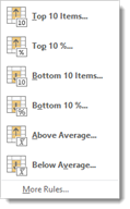
Select if you want Excel to highlight the selected cells that have the top ten values, the top 10% values, the bottom ten values, the bottom 10% values, above average values, or below average values.

We have chosen Top 10%.

We now see the Top 10% dialogue box.

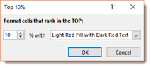
If you want, you can adjust the percentage up or down. You can also change the highlight color for the cells.

Click OK when you are finished.

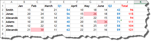
As you can see, our top 10% values were highlighted.

Conditional Formatting Presets

Conditional formatting presets give you additional ways to create visualizations of your data using colors, bars, and icons. These can not only help you visualize your data, they can also dress up your worksheets and make them look more attractive.

To apply a conditional formatting preset, start out by selecting your cells just as we did in the last section.

Return to the Home tab and the Conditional Formatting dropdown box.

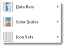
The snapshot below shows the conditional formatting presets. As you can see, there are three different types of presets: Data Bars, Color Scales, and Icon Sets.

• Data bars are bar graphs that appear in cells. The bar graph represents the value in the cell.

• Color Scales change the background color of a cell based on its value.

• Icon Sets adds groups of symbols, ratings, or indicators to cells. 

The Data Bars menu is pictured below.

The Color Scales menu:

The Icon Sets menu:

Applying Data Bars

We have already selected the data in our worksheet.   Now, we want to start applying conditional formatting presets to that data. 

We are going to start out by applying data bars to the cells in the worksheet.

To do this, go to Conditional Formatting under the Home tab, and select Data Bars.

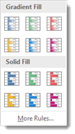
Select the style of data bars that you want to apply.

As you can see, you can choose different colored fills. You can also choose Gradient or Solid. 

We chose the green solid fill, as shown below.

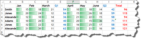
Notice that there is now a bar graph in each cell we selected. The bar graph represents the value inside the cell.  

We can easily look at the bar graphs to see the cell with the highest value, as well as the lowest value.

Applying Color Scales

In addition to bar graphs, you can also apply color scales to selected cells.

In the snapshot below, we have selected our data again.

Go to the Conditional Formatting dropdown menu again, and choose Color Scales.

Choose the color scale that you want to apply to the selected cells.

A gradient color scheme is used for the background colors. Each cell is assigned a background color based on its value. 

For example, take a look at the green cells.   We notice that the lightest green cells, such as F4 and F5 have values of 21 and 20 respectively.   But if we look at the cells that contain darker shades of green, their values are greater.

Applying Icon Sets

Icon sets allow you to add symbols, ratings, or indicators to selected cells.

To apply an icon set to our data, we once again select the cells we want to use.

Next, go to the Conditional Formatting dropdown menu, and go to Icon Sets.

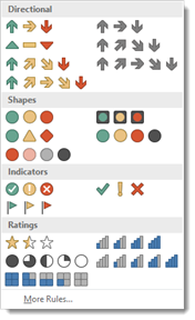
You can add directional icons to your cells. These icons will use direction to show the value of each cell.

You can also add shapes. Shapes will use color to represent a cell.

Indicators will add symbols or flags to your cells. The indicator assigned will be based on the value of the cell.

Ratings will add a visual rating, such as stars, based on the value of each cell.

Let's add a rating icon set to our data.

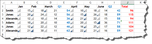
As you can see, Excel placed bars in each cell. The more bars that appear a dark blue, the higher the value of that cell.

Now, let's choose a directional icon set to place in our data instead.

The arrows that point straight up are placed in cells with higher values.   If the arrow points straight down, the cell has a lower value (as compared to the other cells).   The  arrow symbolizes data that is in between the lowest and highest value, and on the low side. The  arrow symbolizes data that is in between the lowest and highest value, but is on the high side. 

Creating Conditional Formatting Rules

So far, we have used predefined conditional formatting rules.   These may be all you ever use, and they may work perfectly for your data.   However, there may be times when Excel's predefined conditional formatting rules are not what you need for your data.   You want to apply conditional formatting, but the rules available just will not work.

Excel 2016 gives you the capability to create your own conditional formatting rules.

To create a new rule, go to Conditional Formatting, and click on New Rule.

You will then see the New Formatting Rule dialogue box.

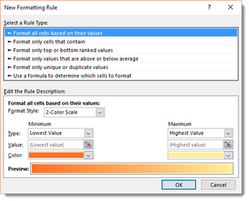
Start out by selecting a rule type.   As you can see, you can choose to:

• Format cells based on their value.

• Format only cells that contain certain criteria.

• Format only top or bottom ranked values.

• Format only values that are above or below average.

• Format only unique or duplicate values.

• Use a formula to determine which cells to format.

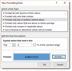
We are going to choose to format the top ranked values, we will select "Format only top or bottom ranked values".

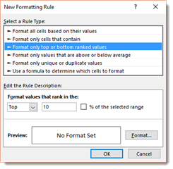
By default, it shows that Excel will highlight the top ten values.

We are going to change this to the top two.

Next, we are going to click on the Format button in the New Formatting Rule dialogue box (pictured above) to specify how cells meeting our criteria will be formatted.

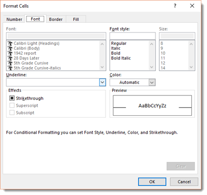
The formatting options presented are the same formatting options available for text, numbers, and cells in Excel. They should be familiar to you. 

Select your formatting options, the click the OK button.

Once you click the OK button, you are then taken back to the New Formatting Rule dialogue box.

Click the OK button again. Your formatting rule is then applied to the selected cells.

Managing Formatting Rules

Once you apply conditional formatting rules to selected data, you can then edit, delete, or apply new rules by using the Conditional Formatting Rules Manager dialogue box.

To access the dialogue box, go to Conditional Formatting dropdown menu, and click on Manage Rules.

You will then see the Conditional Formatting Rules Manager dialogue box.

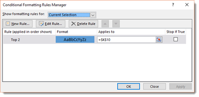
In the Show Formatting Rules For dropdown menu, select what rules you want to see. We have chosen the Current Selection; however, you can also choose the worksheet, as well as other worksheets in the workbook.

Next, there are buttons to create a new rule, edit an existing rule, or delete a rule.

If you want to edit or delete a rule, click on the rule, then click the appropriate button.

Click the Apply button to apply any changes, then click OK.

Clearing Conditional Formatting

If you want to remove conditional formatting from your data, go to Conditional Formatting, then select Clear Rules.

Sparklines represent data in your worksheet. They show the variations or trends in a section of your data, typically within a row.   For example, if you have a worksheet that contains monthly sales in Row A, you could add a sparkline that shows the variations in sales for the months in those rows. 

Sparklines appear as small charts that inhabit a single cell, but they are not associated with Excel's charting feature.   Instead, they are simply a tool you can use to display your data in a way that you can see the variations in it at a glance.  

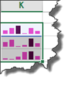
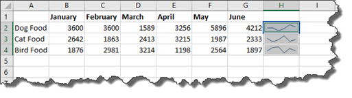
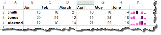
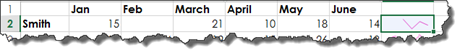
You can see an example of a sparkline under column K in the snapshot below.

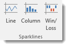
Sparkline Types

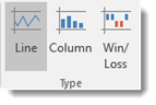
There are three different types of sparklines in Excel 2016.   The type of sparkline you choose will be based on how you want your data displayed in the sparkline. 

The three types of sparklines are:

1.       Win/Loss. This is a binary type chart that will display each data point (or data from a cell) as a high or low block. The Win/Loss sparkline is pictured below.

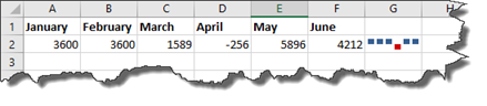
As you can see, the sparkline shows the change each month based on wins and losses. A win is a high block. A loss is a low block. In our example, the low block represents the month of April. 

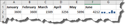
2.       Column. The column sparkline is much like a column chart. It displays the data as columns, as shown in the snapshot below.

3.       Line. The line sparkline is much like a line chart. Each piece of data represented in the line sparkline is represented by a marker (or a dot), as shown below.

Creating a Sparkline

Let's start out with a quick review of how to create sparklines to represent data that you have entered into a worksheet.

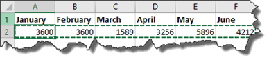
To create a sparkline in Excel 2016, start out by clicking on the cell where you want a sparkline to appear, as we have done below.

Go to the Insert tab and find the Sparklines group. 

Select the type of sparkline you want to add.   We are going to select Line.

You will then see the Create Sparklines dialogue box.

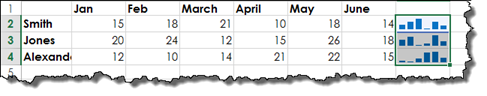
Now select the data that you want represented in the sparkline by highlighting those cells in the worksheet (as shown in the next image).

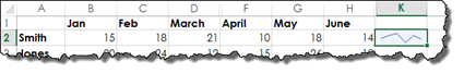
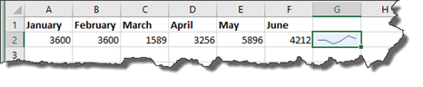
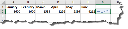
In our example, we have the monthly sales totals in our worksheet. We want our sparkline to be a graphical representation of the monthly sales.   For that reason, we have highlighted the sales for each month.

The range of cells will now appear in the dialogue box, as pictured below.

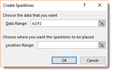
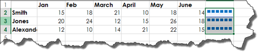
Next, click on the cell where you want to sparkline to appear.   This is the location range.

We have clicked on cell G2.

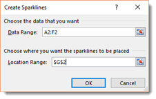
Click the OK button in the dialogue box.

As you can see below, the sparkline appears in the cell that you specified. Notice that the sparkline represents the sales trends as Smith's sales fluctuated from month to month. 

Customizing Sparklines

Once you have added sparklines to a worksheet, you can then alter the design of those sparklines to adhere to the look and feel of your worksheet – or to better suit the data that they represent.

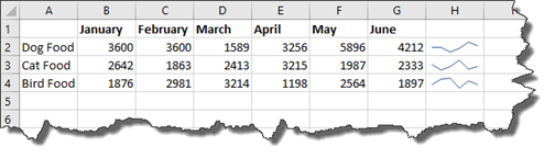
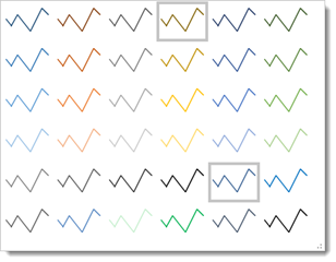
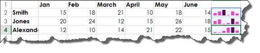
Notice that in the snapshot below that we have added three sparklines.

When we click on the cell that holds the sparkline, the Sparkline Tools Design tab will appear in the ribbon. 

Let's click on cell G2. This cell holds our first sparkline.

When we click on this cell, we see the Sparkline Tools Design tab appear in the Ribbon.

It looks like this:

Changing the Sparkline Colors and Width

From the Sparkline Tools Design tab, we can change the style of the line used in our sparkline by going to the Style group.   Click the dropdown arrow in the Style group gallery to see all your options.

As you can see, you can choose a new color for your sparkline in the gallery (pictured above).

If you do not see a color you want to use, you can click on the dropdown arrow for Sparkline Color.   This is also in the Style group.

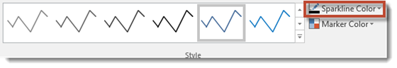
Click the dropdown arrow.

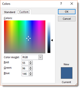
You can pick a color, or you can create your own color by clicking More Colors.

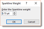
To change the width of the line, click the Sparkline Colors dropdown arrow, then click on Weight.

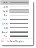
You can select a preset thickness, or you can click on Custom Weight to create your own line thickness.

Changing the Marker Color in a Line Sparkline

From the Style group under the Sparkline Tools Design tab, you can also change the color of the markers in a line sparkline.

To do so, go to the Style group, then click the Marker Color dropdown arrow.

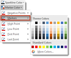
Select Markers, as shown above, then select a color just as you did with the line color.

Highlighting Data Points

You can also customize your sparklines to highlight aspects of the data by applying different colors to certain data points.

You can apply a different color to a high point, low point, negative points, first point, or last point. 

Select:

• High Point to have the highest data value highlighted.

• Low Point to have the lowest data value highlighted.

• Negative Points to indicate negative values.

• First Point to highlight the first data value.

• Last Point to highlight to last data value.

• Markers to mark data points in a Line sparkline.

To do this, go to the Style group under the Sparkline Tools Data tab.

Click the Marker Color dropdown arrow.

Select the point for which you want to apply a different color. We have selected High Point.

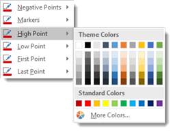
Choose the color you want to apply to the point.

Take a look at our column sparklines with the high point highlighted:

And the low point:

The first point:

And the last point:

Adjusting Axis Scaling

All sparklines use automatic axis scaling. What this means is that the minimum and maximum axis values are determined by the range of data included in the sparkline. This is done by default. However, you an override this feature so that you can control the minimum and maximum axis values. 

To do this, go to the Sparkline Tools Design tab, then the Group group. Click on the Axis dropdown arrow.

NOTE: Sparklines do not show a vertical axis. If you adjust the vertical access, you are adjusting an invisible axis.

Sizing the Cells that Hold Sparklines

You can change the height and width of a cell that contains a sparkline. Just note that if you change the height or width of the cell, the sparkline will adjust in size accordingly.

Changing the Type of Sparkline

Let's say you have added a line sparkline to a row of data.   However, you realize after you have added it that you want to add a column sparkline instead.  

Excel 2016 gives you the ability to change the type of sparkline you have selected after you have already inserted it into your data.

To change the sparkline type, select the cell that contains the sparkline, then go to the Sparkline Tools Data tab.

In the Type group, select the type of sparkline you want to use.

Below are column sparklines.

In the next snapshot, you can see win/loss sparklines:

Grouping Sparklines

You can group sparklines together so that you can make formatting changes to all the sparklines in the group at the same time. For example, you may want to group all sparklines that are in the same row – or the same column – so you can keep their appearance uniform without having to take the time to change the formatting of each one, one at a time. 

To group sparklines together, select the sparklines you want to group by holding down the Ctrl button on your keyboard as you select them.

Next, go to the Sparkline Tools Design tab, then the Group group, as pictured below.

Click the Group button.

The sparklines that you selected are now grouped together.   If you make formatting changes to one sparkline in the group, those changes will be applied to all sparklines in the group.

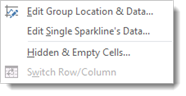
Changing the Data Source for a Sparkline

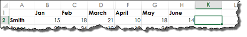
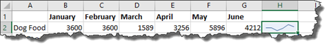
In the sparkline pictured below, we used data from cells B2 through G2. 

To change the data that is represented in the sparkline, go to the Sparkline Tools Design tab, then to the Edit Data group.

Select Edit Single Sparkline's Data from the dropdown menu.

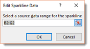
Edit the source data range, then click OK.

NOTE: You can change the data source for a single sparkline or for a group of sparklines. To change the data source for a group of sparklines, choose Edit Group Location and Data.

Edit the data source, then click OK.

Comparing Sparklines in a Group

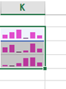
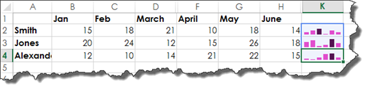
Take a look at our sparklines in the snapshot below.

As you can see, we have chosen the column type sparklines.   We also have the high points highlighted so that the highest data value in each range appears as black bar instead of purple.

• In the Smith row, the high point represents 21.  

• In the Jones row, the high point represents 26.

•  In the Alexander row, the high point represents 22.

We want a way to compare the data that is represented in all sparklines. In other words, we want a way to compare all the sparklines.

The first thing we need to do is group these sparklines together. To do this, select all the sparklines, then go to the Design tab.

Click on the Group button.

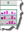
As you can see, when sparklines are grouped together, a blue border will appear around all the sparklines in the group when you click on one of the sparklines.   We clicked on the sparkline in the Alexander row, and a blue border appeared around all the sparklines that we grouped together.

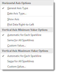
To compare the sparklines, go to the Sparkline Tools Design tab and click on the Axis button.

Look under Vertical Axis Minimum Value Options in the Axis dropdown menu (pictured above).

As you can see, it is set automatically for each sparkline. 

The same is true for Vertical Axis Maximum Value Options.

To be able to compare values in the sparklines, we need to change this to Same for All Sparklines for both the minimum and maximum value options.

By doing this, you can compare the sparklines in the group.

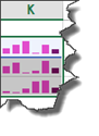
Take a look at our sparklines below.

We can now see that Jones has the highest data point of all three employees, followed by Alexander, then Smith.  

Now you can compare the values in the sparkline to the entire group of sparklines, rather than just the data values that an individual sparkline represents.

Dealing with Empty or Hidden Cells in a Sparkline

If there are data values missing within the range that you have specified for a sparkline, you will see it visualized in your sparkline.

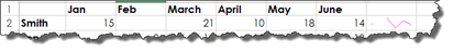
Using our spreadsheet as an example, we have deleted the data value for the month of February for the employee named Smith.

When this happens, the sparkline is interrupted, as shown below.

Because we have the data points visualized (by checking Markers in the Show group under the Sparkline Tools Design tab), we can see the first data point. However, if we did not have the data points visualized, you would likely not even see the data that comes before March, the point where the sparkline resumes after the empty cell.

Take a look below:

That said, you can specify how Excel deals with empty cells and missing values.  

To do this, go to the Design tab again.   Click the Edit Data dropdown arrow.:

Select Hidden & Empty Cells.

You will then see the Hidden and Empty Cells Settings dialogue box.

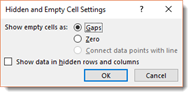
Choose an option.

• Gaps makes it so that if a value is missing, there will not be a connecting line displayed.

• Zero makes it so that when a value is missing, it will be displayed as if the value was 0.

• Connect Data Points makes it so that the missing value is ignored. The existing values will be connected with a line. However, this option is only available with line sparklines.

• Show Data in Hidden Rows and Columns means Excel displays the value even when rows or columns that contain that value are hidden. 

Click OK when you are finished.

Removing Sparklines

To delete a sparkline, simply select the sparkline or group of sparklines that you want to delete.

Click the Clear dropdown arrow under the Sparkline Tools Design tab.   It is located in the Group group.

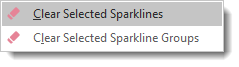
Select if you want to clear the sparklines that you have selected, or clear the selected sparkline groups.

Working with a Date Axis

If you take a look at our worksheet below, you will see that it displays data for sales by date. The dates range from January 4^th to January 18^th. 

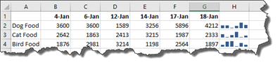
We are using a column sparkline to represent the data.   Each column represents a different date. Since there are six dates displayed, we see six columns in our sparkline. 

This is not a good visual representation.   We can see that our data covers six days by the number of columns in the sparkline, but we can't tell that these days were not consecutive.

To fix this, we are going to change the date axis by going to the Sparkline Tools Design tab, then to the Group group.

Click the Axis dropdown arrow.

Select Date Axis type.

You will then see the Sparkline Date Range dialogue box.

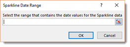
Select the range of cells that contains the date values. We are going to select the six dates in our worksheet.

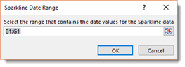
Click OK when you are finished.

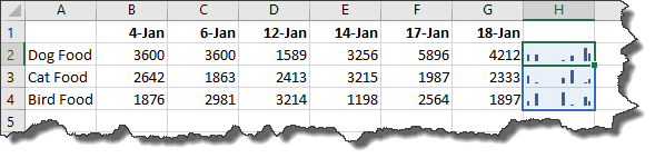
As you can see in the snapshot below, the missing dates are represented in our sparkline.

Refreshing Sparklines When New Data is Added

Worksheets contain data, and data is always changing.   Chances are you will add new data to the beginning or end of the data range used to create a sparkline.   When you add data to the beginning or end of the range, the sparkline does not automatically update to add the new data. To refresh the sparkline, you must go to the Sparkline Tools Design tab, then click the Edit Data.

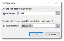
You will see the Edit Sparklines dialogue box.

This dialogue box should be familiar to you.

Select the new range of data, then select where you want the sparkline placed.

Click the OK button when you are finished.

That said, if the data used by your sparkline is in a column that is part of a table, the Sparkline will incorporate new data that is added to the end of the dable. 

Creating Sparklines for Dynamic Ranges

Let's say you are a sales manager for your company. Your job is to track the sales of the products that your company sells. The worksheet you create in Excel may display sales for every day for the past quarter, because you will use those sales figures to create forecasts, goals, and any number of other things.    However, that is the big picture. 

While it is important to track quarterly sales, it is also important that you track the most recent sales.   Perhaps you want to track sales for the most recent seven day period, and you want to be able to easily see the trends for the most recent seven day period in a sparkline. You can do this by creating a dynamic range for the sparkline.

To do this, start out by creating a dynamic range name by going to the Formulas tab, then clicking the Defined Name dropdown arrow in the Define Names group.

You will then see the New Name dialogue box.

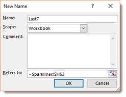
You can name the dynamic range whatever you want. We are going to name ours Last7 since it will represent the last seven days of sales.

In the Refers To field, enter this formula:

=OFFSET ($FirstCellInRange, COUNTA ($Column: $Column) 7 -1, 0, 7, 1)

Let's explain this formula.   We are using the OFFSET function.   The first argument names the first cell that appears in the range of cells. For the second argument, we list the number of sells in the column minus the number that will be returned, minus 1 for the colulmn label. 

Next, go to the Insert tab. Insert a line sparkline.

You will then see the Create Sparklines dialogue box.