In Excel 2016, data functions help you locate specified data from your lists of data. For example, if you have a worksheet that has a list of a thousand of your employees, along with their ages, you can use a data function to find an employee's location in a worksheet. This is easier than scrolling through countless rows. You can also find the employee and then find their age.   In short, data functions give you various ways to search your data.

The MATCH Function

The MATCH lets you check an item against the list, and it will tell you where it appears in the list.

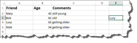
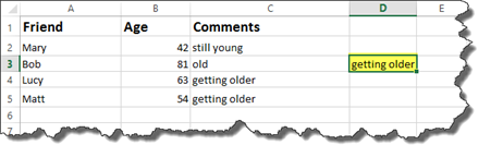
Take a look at our spreadsheet below.

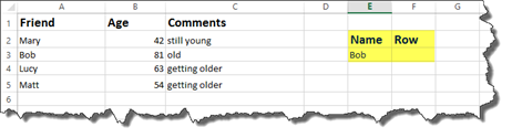
We are going to use the MATCH function to find the row in the list (on the left) where the name Bob is found. 

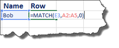
To find this, we are going to type:

The MATCH function asks for the:

• Lookup_value. In this case, that value is E3. This is where we have written Bob's name as the name we will search for. Instead of E3, we could have also typed "Bob" in our formula.

• Lookup_array is the range of cells where the data will be found. We selected the column.

• Match_type is 0 or 1. 0 is an exact match. -1 is less than. 1 is greater than.  

Press Enter.

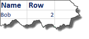
Excel tells us that Bob's name is in row 2. 

Note: If there had been two Bobs in our list, it would only show the location of the first Bob.  The MATCH function only returns the first match.

In our example, we searched for text. The text we searched for was "Bob." 

When you search for text, you will search for the exact value (0) for the match_type.   You may also use wildcards, as we will learn about shortly.

However, if you are searching for numerical data using the MATCH function, -1 would return the first match that was LESS than the value you are searching for. 1 would return the first match that was GREATER than the value you are searching for.  

In the example above, if we replaced Bob with the number 10, a match_type of -1 would search for the first value that was less than 10. 1 would search for the first value that was greater than 10. 

About the Wildcard Feature

As we mentioned, the MATCH function also has a wildcard feature.   The wildcard feature allows you to look for parts of a name.

For example, if we were looking for a name that began with Ma, we could use the MATCH function with the wildcard feature.

The wildcard feature is actually just an asterisk.

Take a look at our formula below:

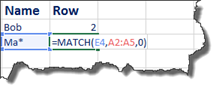
Notice that the asterisk was placed in the cell that we referenced as the lookup_value.

Press Enter.

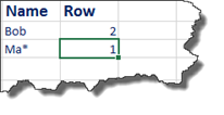
We are shown that a name that begins with Ma is located in row 1.   If we look at our list, this name is Mary.

In addition:

• You can put an asterisk at the beginning of a name. For example, to find names that end with -es. 

• You can put a question mark for a single wild card character, such as Ma?y. 

The INDEX Function

The INDEX function will give you the value of a cell that is at a specified location.

Below, we are going to use the INDEX function.

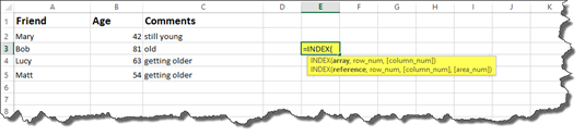
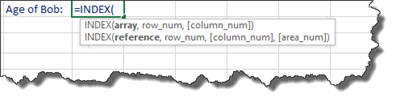
Notice that the INDEX function has two sets of parameters. You can use either one. 

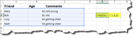
Let's use the first set of parameters first which is INDEX(array,row_num,[column_num]).

For this example, let's say our array is a column of cells. We have selected those cells below.

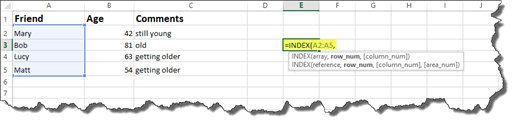
Next, we enter a row number.

We are going to enter 3.

The number three stands for the 3^rd position in the array we selected, or the third row in the array we have selected.

Close out the formula using an end bracket.

Hit Enter.

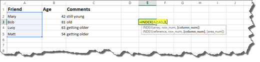
If we wanted to use the INDEX function to find a value in an area (both columns and rows), then we could also use the [column_num] parameter. However, this is optional.

Let's see how it works.   Let's say we want to find a value in a range of cells that contains columns and rows. 

You would enter =INDEX( then select the range of cells for your array. In our last example, we only selected a column for our array, now we select rows and columns.

Next, enter the row number, then the column number. Close out the Formula.

Press Enter.

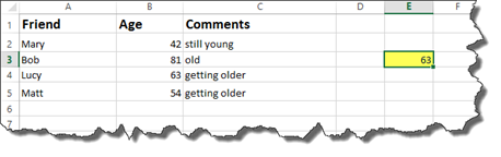
Remember, row 3 is actually position three. Based on our selected array, that is actually row 4 in the spreadsheet. 

Column 2 is actually position two. Position two is the age column. If we scroll down to position three, we can see that the value is 63, the same value that we see returned below.

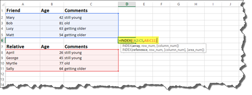
Now, let's look at the second set of parameters for the INDEX function.

The second set of parameters asks for a reference instead of an array.

A reference is a group of arrays.

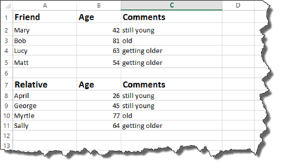
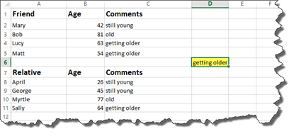
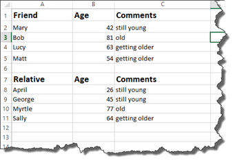
In our worksheet below, we have two different lists. One is for friends. The other is for relatives. We are going to select two sets of arrays. One list will be one array. The other list will be the second array.

Here is how we enter it:

We now have our reference parameter. 

Enter a row number.

Enter a column number.

The area_number parameter is optional.

Close the formula.

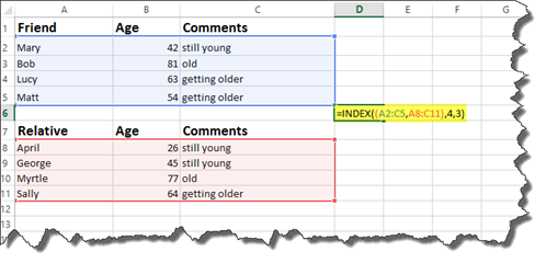
Press Enter.

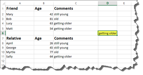
Our results our "getting older." This is indeed row 4, column 3, but that is only for the first array – or area that we selected.

If we want Excel to look at the second area we have selected, we need to use the optional area_number parameter.

We are going to enter 2 for the area_number.   The area_number is determined by the order they appear in the reference section. 

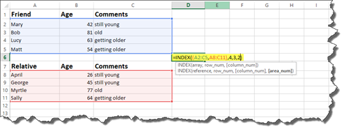
This will return results in the second area, or the area where we have relatives.

Out of Range Requests

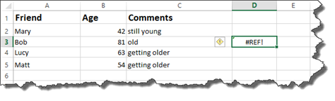
If you use an INDEX function, then enter a row or column number as a parameter, and that row or column does not exist, you will get a #REF error.

Take a look at the snapshot below.

We entered row 6 as the row number.

What we want to do is make that error message look better – and to also better communicate what the problem is.  

We can use an IF statement to get rid of those error messages.  

Let's put an IF statement into our formula.

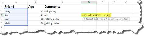
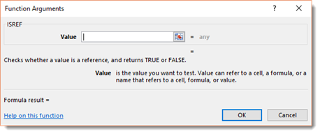
We are going to use the ISREF function to run a logical test.   The ISREF function checks to see if certain cells reference one another.

This is how we would enter it:

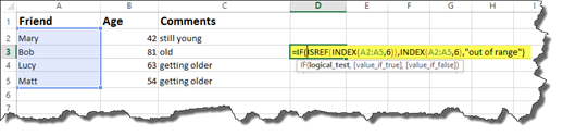
In the snapshot above, you can see what we specify to appear in the cell for the value if true, as well as the value if false.

Press Enter.

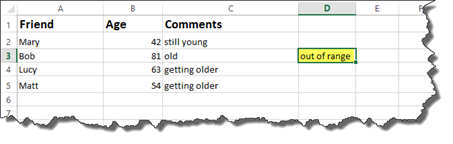
We no longer have a #REF message in the cell.   Now it simply says out of range.

You can also find the ISREF function by going to Formulas>More Functions>Information>ISREF.

The Functions Arguments dialogue box is shown below.

The CHOOSE Lookup Function

The CHOOSE function is another lookup function. Whereas the INDEX function deals with ranges or groups of ranges, the CHOOSE function deals with individual cells.

You can see the parameters for the CHOOSE function highlighted below.

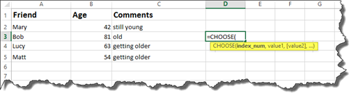
Index_num refers to the number of the item in a comma separated list of cells.

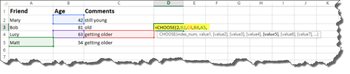
In our worksheet, we want to search the 2^nd item in our comma separated list. 

We would enter the number 2, then select the cells we want to look up, separating each of them with a comma, as shown below.

These are value1, value2, value2, etc, all the way up to value254.   This means you can have up to 254 values.  You can also have groups of ranges.

Close the brackets when you are finished entering values.

Hit Enter.

We can see our returned value is "getting older."   This is indeed the second value we selected.

Using the MATCH and INDEX Functions Together

When you use the MATCH and INDEX functions together, you can use them as an alternative to VLOOKUP and HLOOKUP.   In fact, they can be quicker and easier to use.

Let's look at how to use the MATCH and INDEX functions together.

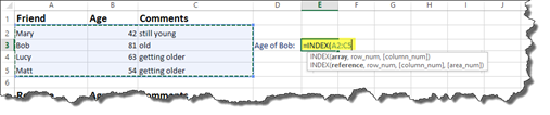
Take a look at our worksheet below.

Let's say we want to determine the age of Bob.

We start out using the INDEX function.

Next, we select the array of cells.

Enter a comma, then the match function.

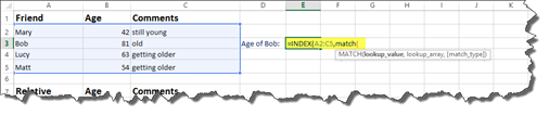
Now we enter the formula for the MATCH function.

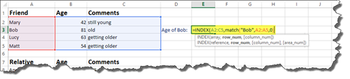
In the snapshot above, the lookup_value is "Bob." We selected the lookup_array, which is A2:A5. We entered 0 because we want an exact match.

Now let's enter a comma and return to finish the INDEX function.

We need to specify which column. This is another MATCH function.

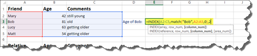
We want to search column 2.

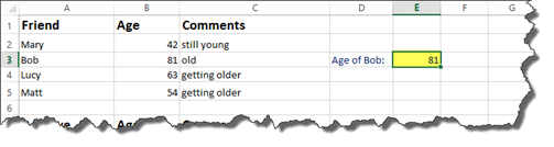
Close the brackets, then press Enter.

NOTE: If you needed to, you could use another MATCH function for the column parameter as well. In other words, you can use more than one MATCH function when using INDEX and MATCH together.

The IS Functions

In Excel 2016, the IS functions return logical true or false values.   IS functions are used to get information regarding a value before it takes another action, such as solving a formula.   In conjunction with IF statements, we told Excel what we wanted to appear on the screen if the outcome was true or if it was false. In short, IS functions check for errors.

The ISERR and ISERROR Functions

As we just said, IS functions check for errors.  

Now let's take a look at how to use them.

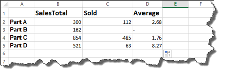
Take a look at our worksheet below.

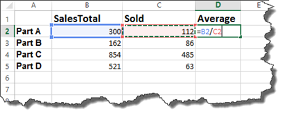
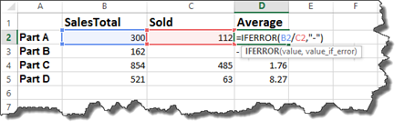
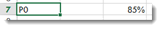
In this example, we have four different parts that were sold. The SalesTotal column shows the dollar amount earned from all sales. 

The Sold column shows how many were sold.

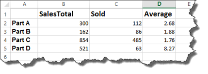
In the Average column, we have entered a formula to produce the average price per product sold.

Let's press Enter, then complete the average for each part.

If we remove a value from the SOLD column, we will get an error message.

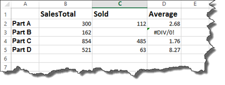
Excel is letting us know we are trying to divide by 0.

To prevent us from seeing those unattractive error messages, we can use the ISERR function to check for errors as we calculate formulas.

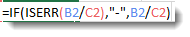
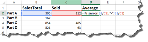
Instead of entering =B2/C2 as we did in cell D2 to calculate the average, we will instead enter the ISERR function along with the formula.   If there is an error, we want a dash to appear. If there is not an error, we want Excel to calculate the formula and display the results.

Let's look at how we enter it. 

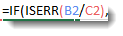
First, we enter =IF(iserr for the ISERR function, then an open bracket.

Enter the formula that you want to calculate.

Ours is C2/D2.

Close the brackets.

Enter a comma.

What we have said is this: If there is an error when you divide C2/D2…

Next, we have to tell Excel what to do.

If it is true, and there is an error, we want Excel to display a dash.

If it is false, and there is not an error, we want Excel to calculate the formula and display the results.

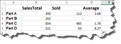
Press Enter, then finish completing the average for each product.

The error message that was showing for Part B is now a dash.

The ISERROR function works in the same way.

Hit Enter. 

You can then finish the worksheet by dragging the handle in the lower right corner of the cell.

As you can see, when there was an error, Excel returned a dash. 

NOTE: You can also find the IS functions under Formulas>More Functions>Information

The IFERROR Function

The IFERROR function is a shortcut, per se, to the ISERR and ISERROR functions. 

With the IFERROR function, you simply enter =IFERROR, then the parameters in brackets.

The first parameter is the value that you want to test for an error.   If we use the previous worksheet, it is C2/D2.  

Next, is the value_if_error.   Enter what you want displayed in the cell if an error is found.

You can see the IFFERROR function below.

Press Enter.

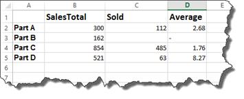
If you look at our worksheet, you will see the IFERROR put a dash in the cell where there was an error.  

The OFFSET Function

The OFFSET function returns the address of a cell or range of cells by using a reference cell. When you use the OFFSET function, you select a cell or range of cells that are offset from a location.

Let's take a look at the OFFSET function in an actual worksheet to better understand the purpose it serves.

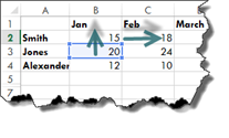
Here is the worksheet.

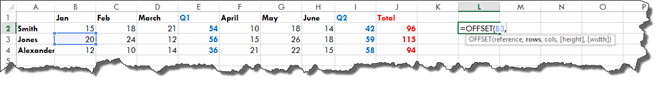
Now let's enter in our formula.

The first parameter asked for when you use an OFFSET function is a reference. This is the starting point.   After you enter the reference, Excel wants to know how many rows and columns offset from the starting point that you want to be.

Let's choose our reference.

Now we have to decide how many rows offset we want to be. This can be a positive or negative number. A positive number takes us down, a negative number takes us up. 

Let's use -1.

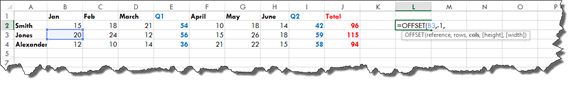
This will move us up one cell on the worksheet.

Next, enter the number of columns. A negative number will move to the left. A positive number moves to the right. You can also enter zero to stay in the same column. 

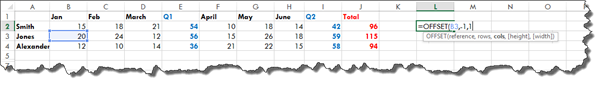
The final two parameters that you can enter are optional.   They are height and width. We will talk about those in another example.

NOTE: You can also enter formulas for any of the parameters to perform a calculation that determines how far you move from the starting point.

For now, add a closing bracket, then press Enter.

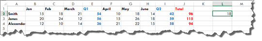
If we count cells from out starting point, we can see that is up one cell and to the right one cell.

In our example, we offset a single cell.   If we want to offset an entire range, we will use the height and width parameters we mentioned just a second ago.

Let's take a look at how to do it.  

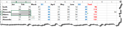
As you can see, we have expanded our worksheet.

We start off the same as we did with the last example by choosing the reference cell, then the number of rows and columns.

However, now we are going to enter how many rows to include (height) and how many columns to include (width).

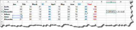
We have extended our range by two rows and two columns.

The offset is now defining a range.

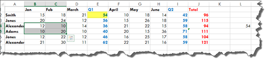
Press Enter.

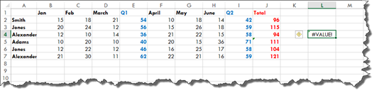
This causes us to get a #VALUE! error because Excel does not know what to do with the range.

To eliminate the error, the range can be embedded in a sum.   It can also be embedded in any other type of function, such as COUNT, MIN, MAX, etc.

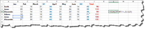
Press Enter.

We now get 54. 

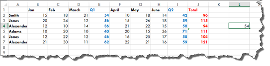
54 is the sum of the four cells selected below that define our range:

It is the total shown in our highlighted cell below.

Creating a Dynamic Named Range

At first glance, it is easy to wonder in what situation you would ever use an OFFSET function. A real world example of using the OFFSET function is in creating dynamic named ranges, as we are going to show you how to do.

Take a look at our invoice below. 

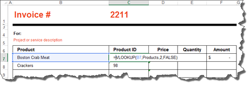
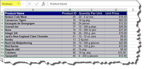
If you also remember, we named our data range in our products worksheet, shown below.

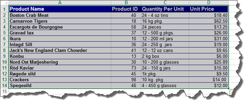
However, when we tried to add a new product at the end of the range, Excel did not include it in the named range. As a result, we could not enter it into our invoice.   At that time, we decided to insert the new row in the middle of existing rows so that it would be included in the named data range. 

Now, we are going to solve that problem. We are going to use the OFFSET function to make it so that our named range dynamically increases in size.   This means if we add a new row to the bottom of the named range, the named range will automatically expand.

Our named range is currently titled Products.

Let's learn to turn it into a dynamically named range.

Click the Name Manager button under the Formulas tab.

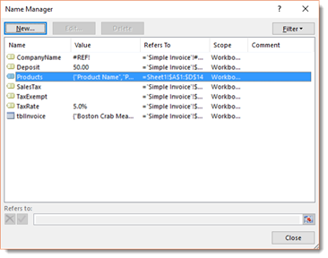
We have clicked on Products.

Go down to the Refers To field at the bottom of the dialogue box.

It is there that we can start to enter our OFFSET function.

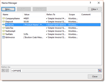
Let's finish adding it.

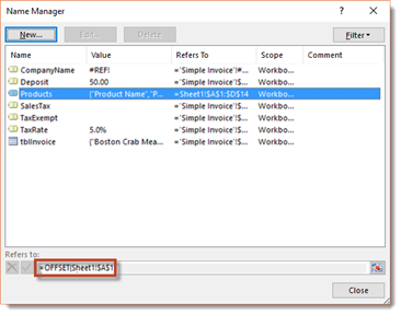
The first thing we entered was our reference. Our reference is our worksheet since this worksheet contains our product list. This is titled Sheet1. We put an exclamation point to let Excel know we are referencing the worksheet. Then, we put the cell that we are referencing, which is the very first cell in the worksheet.

Now we have to tell Excel how many rows we would like to move. We want to enter 0.   We also want to enter zero for the number of columns.

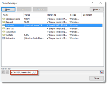
We are not trying to offset the starting point; instead, we are using it to highlight a range.

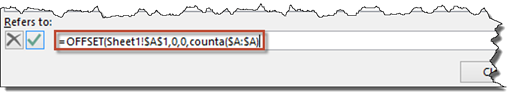
Now we have to enter the height – or how many rows. 

Instead of trying to count them on the worksheet, we will use the COUNTA function. The COUNTA function counts the number of cells that have data. We are going to specify that it count the number of cells in column A.

Next, we add in the width – or the number of columns. We can use another COUNTA function, but since, in our example, we are unlikely to add columns, we are just going to add the number.

Enter a closing bracket.

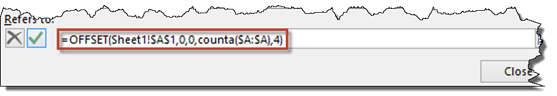
Press the green checkmark button to the left of the formula, then press Close.

Now if we add rows to the product list, it would automatically be included in our dynamic name range.

Creating a Dynamic Formula Using the INDIRECT Function

There might be times when you do not have the actual cell to reference, but you have a cell with a reference to the actual cell in it. This is where you would use the INDIRECT function. 

That may sound confusing.

To show you what we mean, take a look at our worksheet below.

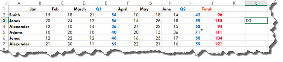
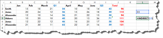
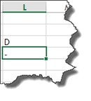
In cell L3, we are referencing cell D3.

We want the value of cell D3 to appear in cell L5. 

The easiest thing to do, especially in very large worksheets, would be to use cell L3 to reference cell D3.

Let's try to do that.

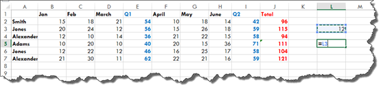
Press Enter.

As you can see, Excel returns D3.

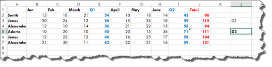
That is not what we want. We want the value of the referenced cell.

To get that, we will use an INDIRECT function.

The first parameter is the reference, which is cell L3, as shown below.

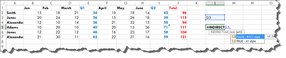
Next, you can decide the optional parameters. As you can see above, we can choose either FALSE or TRUE. FALSE means what we reference will be interpreted as R1C1 – or row 1 column 1. TRUE means it will be interpreted as A1, which is a cell.  

We want true since we are referencing a cell.

TRUE is the default choice, so you do not need to actually enter TRUE. You can just enter a closing bracket if you want.

Press Enter.

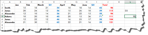
You can now see the value of cell D3 in cell L5.

We are essentially using cell L3 to link to D3.   The INDIRECT function picks up whatever cell reference we have in L3 and displays the value of that cell.

We can now change the cell reference in L3, and it will display the value of that cell in L5. 

INDIRECT functions can be used inside other functions as well.   You can also use them to select and create whole ranges.

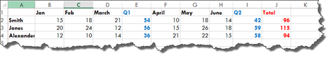
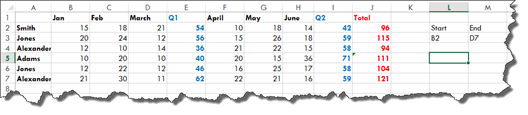
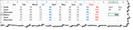
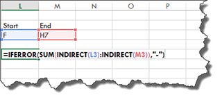
Let's say we want to add a range of cells.   The start cell – or where we want the range to start-- is B2. The end cell – or where we want the range to end – is D7. This will effectively add the total sales for Q1.

In our worksheet below, we have entered the start and end cells.

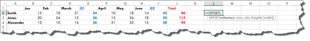
Now let's enter it into cell L5. 

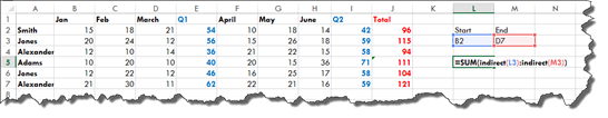
In the example above, we used SUM, but you can use any function that you want.

We have instructed Excel to add the values of the cells referenced in L3 and M3. Right now, L3 and M3 reference B2 and D7 respectively.

Press Enter.

This is the total of our Q1 sales.   If you want, you can double check this by adding up the totals in the Q1 column.

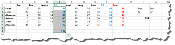
As you can see, it equals 294.

Now, we can go back to L3 and M3 and change the cell references. Let's say we want the total for Q2.

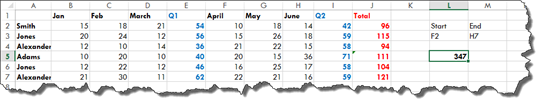
It now gives us the total.

INDIRECT Errors

With INDIRECT functions, if you add a cell reference that is not actually a cell reference, you will see the #REF error.

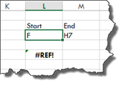
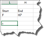
For example, instead of entering F2 as our starting point, we have entered just F below. That is not an actual cell reference. A cell reference needs a row and column.

We get the #REF error message.

We can use the IFERROR function that we learned about earlier in this article to determine what is displayed if there is a #REF error.

All we need to do is enter =IFFERROR( before our INDIRECT function, as shown below, then specify the message that is displayed if there is an error.

Press Enter.

Let's use a simpler example so you can see exactly how the IFERROR function is added.

Let's use our earlier example when we simply reference cell D3, except we are going to make it so we get an error.

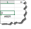
Let's double click on the #REF error, and add the IFERROR function.

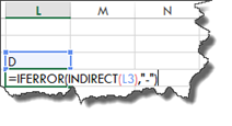
We have essentially told Excel that if there is an error with the INDIRECT function, to display a dash.

Press Enter.

The CELL Function

We have learned to create dynamic formulas and dynamic named cell ranges. However, we can also dynamically determine the name of a workbook or worksheet using the CELL function.

Let's start by dynamically generating the name of the workbook.

In the worksheet, we are going to enter the CELL function.

When we start to enter the CELL function into the first cell in our worksheet, we notice it gives us a lot of information from which to choose.

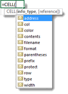
We are going to name our new workbook, so we will choose filename.   We will add a sheet name later, but that has to be calculated.

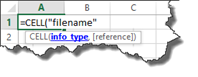
Now we can add reference, which is an optional parameter. 

NOTE: If you have not noticed yet, optional parameters are always in []. 

Enter a closing bracket, then press return.

We see the path to the file. 

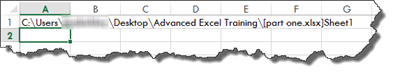
Using the CELL function above, we determined the file path.

Now, we will now create a dynamic formula to extract the sheet name from that path.

To do so, we are going to enter the formula below.

Take note of the different functions we have used.

Now, push Enter. When we do, we see the name of our worksheet displayed in the cell.

If you rename the worksheet in the tab, the worksheet name in the cell will also change.

Next, let's say we want to see the name of the workbook. We know how to display the path, but we just want to see the file name – or workbook name.

We enter the formula below:

Then push Enter.

Other Information Available in the CELL Function

Here is a list of some of the other information you can choose with the CELL function.

• COL displays the column number of the referenced cell.   You need a cell reference for this. Remember, the cell reference was optional with the workbook name.   If you reference cell C3, Excel will display 3. C is the third letter in the alphabet.

• ROW displays the row number of the referenced cell. Again, you will need a cell reference.

• WIDTH displays the width of the referenced cells in pixels. 

• ADDRESS displays the absolute address of the referenced cell.

• COLOR displays the value 1 if the referenced cell is formatted in color for negative values. Otherwise, it shows 0.

• CONTENTS displays the value of the upper left cell in reference.

• FORMAT displays a text value that corresponds to the number format of the cell. The text value for a percentage format is shown below.

• PARENTHESES displays a 1 if the referenced cell is formatted with parentheses for positive or all values. Otherwise, it is 0.

• PREFIX displays a text value that corresponds to the label prefix of a cell.

• PROTECT displays a 1 if a cell is locked. Otherwise, it displays a zero.

• TYPE displays a text value that corresponds to the type of data in a cell. "b" is returned for blank or empty cells. "l" is returned if it contains a text constant. "v" is returned for all other types of cell content.