We are going to continue to explore macros in this article and learn more about creating and working with them.
Formatting with Macros
Formatting cells in workbooks can be a tedious process, especially if you have to format each worksheet in workbooks that you create. To save time and make things easier, you can use macros to format cells and worksheets simply by creating macros that do all the formatting for you. This way, you only apply the formatting once. After that, all you have to do is run the macro.
A macro can contain as many steps as you want it to contain. You can create a macro that changes the font type, color, and size, then also applies cell formatting and row and column sizes. In essence, you can create macros to do all the formatting for you.
We are going to create a macro that does the following things:
1. Changes font type, size, and color.
2. Sets a theme (under the Page Layout tab).
3. Formats the cells to Number with three decimal places.
4. Creates a table in the worksheet.
We are going to call this macro salesWorksheetFormatting.
Notice that we are storing this macro in our personal macro workbook. This way, it is available in all workbooks, and we can use it no matter what workbook we have open.
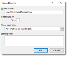
Click OK.
We can then record our macro.
Remember to stop recording when you finish all the steps involved in your macro.
Switching Between Scenarios with Macros
If we go to the Data tab, click the What-If Analysis button, then click on the Scenario Manager, we can see all the scenarios we have created.
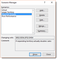
We can select any of these scenarios, then click Show to see the scenario in our worksheet.
If we want to see another scenario, we go back to the Scenario Manager, select the scenario we want to view, then click the Show button again.
This is a lot of clicks.
Instead, we can create a macro for each scenario and add a keyboard shortcut for each macro that we create. That way, we can view a scenario simply by using a keyboard shortcut.
To create a macro for a scenario, go to the Developer tab and select Record Macro.
Name the macro so that you know which scenario it is, then specify a keyboard shortcut.
You will want to store the macro in the workbook.
Click OK, then record yourself opening up the Scenario Manager, selecting a scenario, then clicking the Show button.
Stop recording when you are finished.
You can now view that scenario by running the macro.
Switching Between Custom Views with Macros
In addition to creating macros to view scenarios, you can also create macros to access custom views.
Go to the View tab and select Custom Views.
You will then see the Custom Views dialogue box.
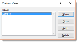
Select a custom view.
If you click the Show button, the custom view will appear in the worksheet.
Instead of having to click the View tab, click the Custom Views button, then click the Show button, you can instead create a macro with a keyboard shortcut that will do all of this for you.
To create the macro, click the Record Macro button under the Developer tab. Name the macro, then assign a keyboard shortcut to it. You will want to store the macro in the workbook.
Click OK, then record yourself going to the View tab, clicking the Custom Views button, then clicking the Show button.
Remember to stop recording when you are finished.
You can now switch to that custom view by simply running the macro.
Using Worksheet Buttons to Trigger Macros
That said, the problem with creating keyboard shortcuts to trigger macros is that, if you have a lot of macros, it can be hard to remember what keyboard shortcut triggers what macro.
Imagine having twenty macros for one workbook, then trying to remember which macro triggers cell formatting. It can be impossible and actually make things more complicated. Macros are supposed to make things easier.
Instead of creating keyboard shortcuts, you can create worksheet buttons instead.
A worksheet button is just as it sounds. It is a button that you place in your worksheet. When you click on that button, it triggers a macro.
To create a worksheet button that will trigger a macro, click in the worksheet where you want to place the button.
Go to the Developer tab. Click the Insert dropdown arrow.
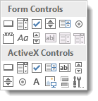
The first icon in the top left corner is a button. Click on the button icon.
Your mouse cursor now is a crosshair.
Click and drag to draw the button.
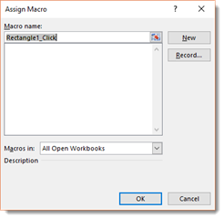
When you release your mouse, you will see the Assign Macro dialogue box.
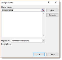
Click on the macro that you want to assign to the button.
Click OK.
The button then appears in the worksheet.
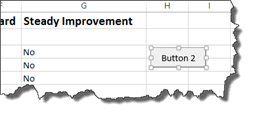
Now you can rename the button. It is recommended that you give the button the same name as the macro or a name that will remind you what the macro actually does.
You can also drag on the button handles to resize it.
When you are finished, click in the worksheet.
The button is now clickable.
Now, whenever you click on the button, it will run the macro.
Customizing Buttons and Other Shape Triggers
You can apply some customization to worksheet buttons and other shape triggers.
To apply customization, select the button. To do this, you will have to right click on it. If you just left click on it, it will run the macro. Instead, right click on it, then select one of the options in the context menu.
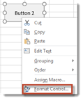
We are going to select Format Control.
This brings up the Format Control dialogue box.
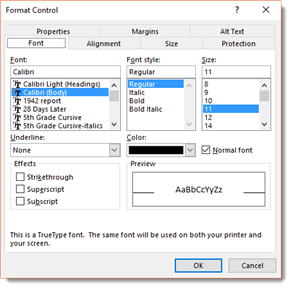
You can click through the tabs to apply different formatting options to your button.
-
The Font tab gives you options to format the text on your button.
-
The Size tab allows you to change the size of the button.
-
The Alignment tab allows you to align the text on the button.
-
The Protection tab allows you to lock an item or lock the text.
-
The Properties tab allows you to control the positioning of the button.
-
The Margins tab allows you to set margins inside the button.
-
The Alt Text tab shows you the label for the button.
Apply any formatting that you want using this dialogue box, then click OK when you are finished.
If you noticed, the one thing you could not change was the color of the button. When we go to the Developer tab to insert a button, we are left with very few formatting choices. For example, grey is the only color of button we can insert, and it is always going to be either a square or rectangle shape.
If we want to use buttons that have different colors and styles � or even use other shapes as buttons, we need to first create a shape and format it.
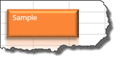
Click the Insert tab, then go to Shapes. Select the shape that you want to use, then drag to draw it on your worksheet as we have done below.
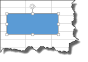
We have chosen to use a rectangle. However, you can use any shape. It does not have to be a rectangle.
The Drawing Tools Format tab is now open on the Ribbon.

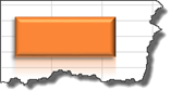
Apply a shape style to the shape if you want. You can also change the shape fill and outline colors. In addition, you can add effects such as a drop shadow.
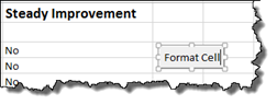
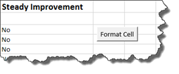
Our shape is shown below.
Next, right click on the shape and choose Assign Macro.
Select the macro that you want to assign to the shape, then click OK.
That macro is then assigned to the button. Whenever you click the button, the macro will be triggered.
Now, right click on the button and choose Edit Text. Add a text label to the button so you know which macro will be triggered when you click on it.
Assign a Macro to a Ribbon Icon
You can also add buttons to the ribbon that will trigger macros. To do this, first go to File>Options.
Click the Customize Ribbon tab on the left hand side of the Excel Options dialogue box.
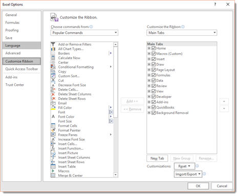
From the Choose Commands From dropdown menu (where it currently says Popular Commands), choose Macros.
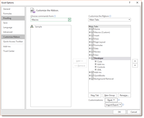
You can now see your macros.
Go to the Customize the Ribbon section of the Excel Options dialogue box. This is on the ride side of the dialogue box.
Choose the tab where you want to place your macros by clicking on it. Do not uncheck the other tabs. This will cause them to not appear on your ribbon.
We are going to choose the Home tab.
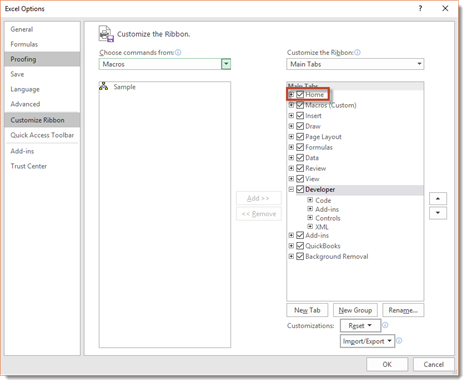
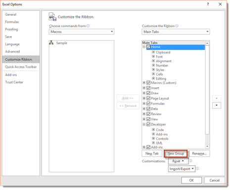
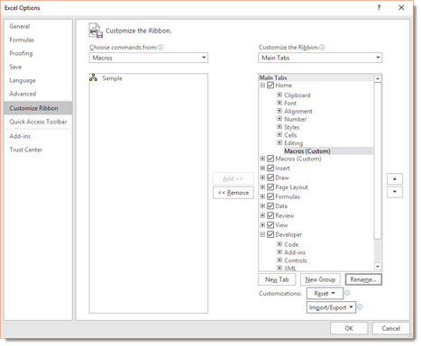
Click on the Home tab to see the groups that are currently under the Home tab. You will have to place your macros in a group under the Home tab. However, you can't place the button in an existing group.
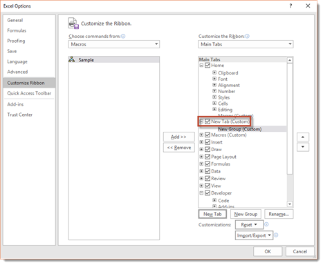
Instead, you have to click the New Group button, as pictured below.
You will then see New Group (Custom), as highlighted below.
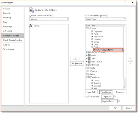
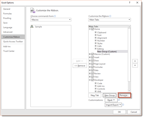
Make sure New Group (Custom) is selected.
Next, click the Rename button that appears to the right of the New Group button.
You will then see the Rename dialogue box.
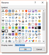
Rename the group. We are naming ours Macros.
Click OK.
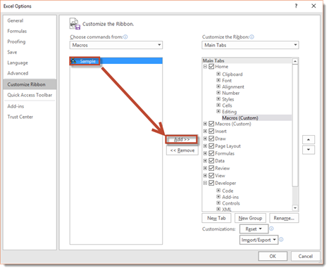
Now, select the macro that you want to add to the group. You will select it from the field on the left, then click the Add button that is between the two fields.
Click the Rename button again.
Click on a symbol to represent the macro. You can also rename it if you want.
Click OK.
When you have added all your macros and selected symbols, you can click OK to leave the Excel Options dialogue box.
Take a look at your Home tab. You can see our new Macros group to the far right on the ribbon.
NOTE: Typically, you will want to use macros that are stored in your personal macro workbook for this. That way, whenever you open Excel, those macros are on your Ribbon and available to you.
Creating Your Own Tab on the Ribbon
In addition to adding macros to an existing tab, such as Home as we did in the last section, you can also create your own tab just for your macros.
To do this, go back to File>Options>Customize Ribbon.
Click New Tab, as shown below.
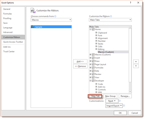
Our new tab is then visible.
Click the Rename button, as we did in the last section.
Name your new tab, then click OK.
Now you can name the group that is included in the tab by default. Right now, its name is New Group.
You can also add more groups by clicking the New Group button.
Next, add macros to the group.
When you are finished, click OK.
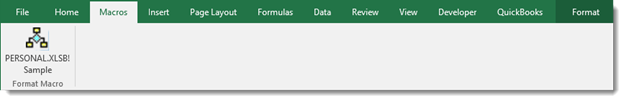
You can then see the Macros tab in the Ribbon.
If we click on the Macros tab, we can see our group.
Editing Macro Code
We do not recommend that you ever attempt to edit the Visual Basic code for your macros. However, just in case you ever need to, we will show you the basics that you need to know in order to be able to make minor changes.
Just be warned, anything outside of the basic editing that we will teach you is a task best left for experienced programmers and not for the typical Excel user. If you mess up the code, you will require the assistance of a programmer to fix it, or you will have to re-record the macro.
To view and edit macro code, go to the Developer tab and click the Macros button.
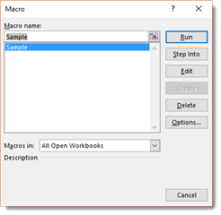
Select the macro that you want to view and edit, then click the Edit button.
NOTE: If you are going to edit code in a macro that is stored in your personal macro workbook, you will need to unhide the workbook first.
Once you click the Edit button, this is what you will see:
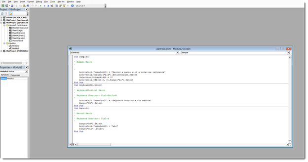
The macro code is shown below.

At the top you see Sub Sample. Sub is for subrooting. Then you see the name of your macro.
At the end you can see that the subrooting is ended. It says End Sub.
Everything in between Sub and End Sub are instructions that the macro will carry out.
Any line where you see an apostrophe at the beginning, followed by green text, are comments. They are not actionable code. You can add more comments if you want. This is very basic, and you are not going to hurt anything by doing this.
Now let's look at the actual code, which is anything in black font that is between Sub and End Sub.
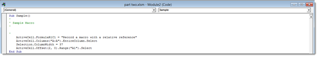
You will see that some of the code appears between quotation marks, such as "Record a macro with a relative reference." This is actually the text that appears in our worksheet when we run the macro. If you want, you can edit text that appears between quotation marks. Again, this is easy enough, and you do not do any damage.
Other things that may appear in your macro that you can easily change are:
-
Font type. Just type in a new font type, such as Arial.
-
Font size. Enter a new font size, such as 14.
-
True/False arguments. You can change an argument from True to False, then vice versa.
-
Range. If the range is .Range("A1"), you could change it to another cell, such as A2.
-
Active Cell. Right now, the active cell appears as ActiveCell.FormulaR1C1. R1C1 stands for row one column one. You could change this to R2C2, for example.
If you recognize anything else and feel comfortable changing it, then you can try to do it. Just remember that you may damage the macro in the process and be forced to re-record it.
When you are finished, simply X out of the window by clicking the X in the top right corner. You do not need to do anything to save the changes. You can then run the macro whenever you want.
Adding a Confirmation Box to a Macro
Although it is not advisable that you attempt to edit the code for your macros, there is a circumstance when you will be required to edit that code. If you want to add a confirmation box to a macro, you will have to edit the code in order to create that box.
A confirmation box is a box that will ask you if you are sure that you want to run a specified macro. This is especially helpful to have if you create a macro that deletes cells or data.
Let's show you how to do this.
Go to the Developer tab and click on the Macros button.
Select a macro for which you want to create a confirmation box, then click the Edit button.
You will then see your code.

To create the confirmation box, we need to start out by adding an If statement. Click at the beginning of the first line of code. Push the spacebar a few times. Then, click to put the cursor above the first line of code. The next snapshot will show you what we mean.
Once you have done that, we can start to enter the code.
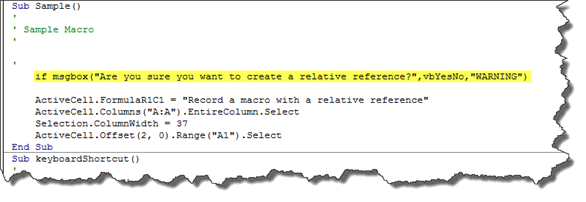
The first thing we type is "if" then add a space, then type "msgbox" to create the confirmation box.
Add an opening bracket, as shown below. We are then told what we need to enter next, as shown below.
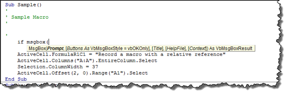
The first thing to enter is a prompt. This is the text that a user will see in the confirmation box that asks them a question.
Type in that question. Any text that will appear inside the confirmation box goes in quotes.
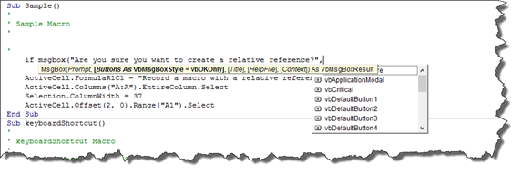
We have customized our prompt to our macro, but your prompt can be anything you need it to be.
Next, select the buttons. We want Yes and No, so we scroll down in the button dropdown menu.
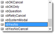
Double click on the button you want to add. It will appear in your IF statement. Add a comma after it.
Next, you can add an optional title to your dialogue box. We are going to enter "Warning."
You do not need the rest of the parameters for a confirmation box.
Add a closing bracket to your IF statement.
We highlighted our IF statement in the snapshot below.
Next, add an equal sign after your closing bracket.
You will see another dropdown menu.
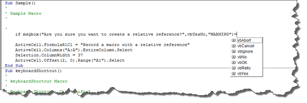
Double click on VBYes in the dropdown menu. This lets Excel know to display the confirmation box. If the answer clicked on in the confirmation box is YES, then to run the macro.
Add a space, then type "then."
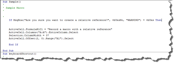
Press Enter.
Next, at the end of your macro, but before the End Sub, type "End If" as we have done above.
Press Enter.
You can now X out of the code window.
Go ahead and run the macro for which you created the confirmation box.
You will see the confirmation box appear on your screen. It will read, "Are you sure you want to create a relative reference?"
We are going to click Yes.
When you click Yes, the macro runs.