Excel 2016 offers a plethora of mathematical functions that you can use. Functions are used to create formulas. In this article, we are going to start talking about some of the more basic functions, as well as teaching you to use them.
The Basic Excel Functions
Before we start to delve into mathematical functions in Excel 2016, let's start out by reviewing the very basic mathematical functions that you are probably already skilled at using.
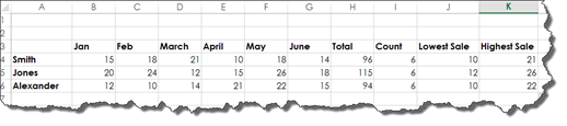
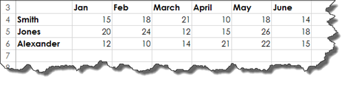
In the snapshot below, we have sales data for a few months' period.
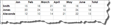
In the Totals column, we want to add the sum of sales for each employee.
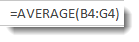
To do this, type in the cell: =sum(
Next, highlight the cells you wish to use to produce the sum.
Now, place the end bracket (parentheses at the end), then press Tab on your keyboard.
You can also click in the cell where you want to place the total (in our example, H4), highlight the cells you want to use to produce the sum, then click the Formulas tab. Click the AutoSum button.
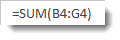
This is how your formula should look in the Formula Bar:
We can now add sums to the rest of the cells in the Totals column.
To do so, we can click the little handle at the bottom right corner of the cell where we just entered the function.

Drag the handle down to select the rest of the cells where you want to copy the same function.
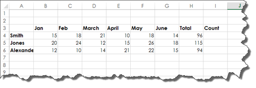
Excel 2016 then produces the sum for each of those rows for you.
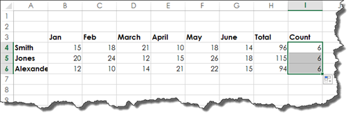
Once we are finished with totals, we are going to add a new column called Count, as shown below.
To enter the count function, type =count( into cell I4, then drag over the cells to include. Enter in the close bracket (parenthesis). Hit Tab on your keyboard.
Excel 2016 then counts the total number of months in that row.
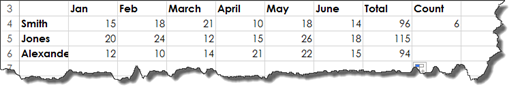
Once again, select the cell (I4) and drag the handle to enter the count for each subsequent row.
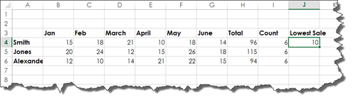
Next, let's search for the Lowest Sales column. We will use the MIN function to find the lowest sales value for the selected data.
The formula looks like this: 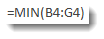
We can now see the lowest sale in our spreadsheet.
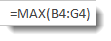
Now let's add a column called Highest Sale and use the MAX formula.
It looks like this:
Take a look at our data below:
Average: Mode, Median, and Mean
For any of your math buffs out there, you know that when we talk about averages in mathematics that there are three different terms: mode, median, and mean.
-
Mode is the most frequently occurring value in a range.
-
Median is the middle-most value in a range.
-
Mean is the total of the values in a range divided by the number of values.
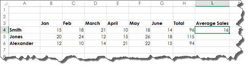
The Mean function in Excel is Average. Here is the formula:
As you can see, we averaged the sales for each month in our worksheet below:
The function for mode is shown below.
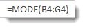
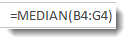
And the formula for median:
The SUMIF Function
The SUMIF function will total the cells in a range that you have selected using criteria that you specify.
Using our worksheet below, we want the total amount in sales for all sales that are greater than 11. You can use any comparison operator that you want in SUMIF functions. We are just going to use greater than.
First, we click on the cell where we went the results to appear.
Next, we go to the Formulas tab, click on the Math & Trig button, then scroll down until we see SUMIF.
Click on it.
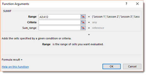
You will then see the Function Arguments dialogue box.
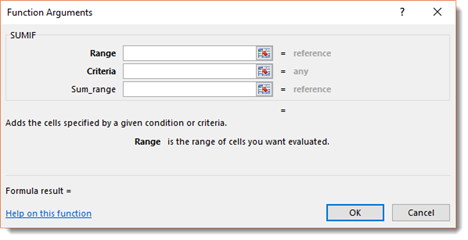
In the Range field, highlight the range of cells that you want to evaluate. This is our sales for the employee Smith.
In the Criteria field, enter the criteria. Ours is <11.
NOTE: If you are writing the formula in the cell, you must use quotations around the criteria: "<11"
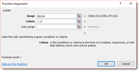
We will look at the Sum Range field in a minute. For now, we just want to see the total of sales for all sales that are greater than 11.
Press OK.
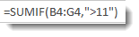
Here is the formula in the Formula Bar:
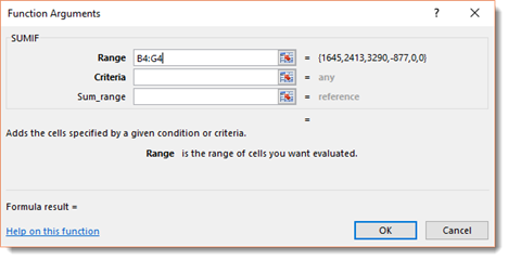
Now let's look at the Function Arguments dialogue box again. Let's talk about the Sum Range field.

The first range in this dialogue box (Range) is for the criteria, and the second range (Sum Range) if for summing. This allows you to use one column or row as the criteria.
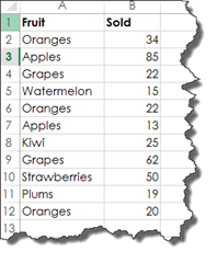
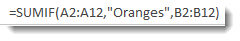
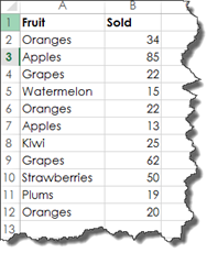
For example, using the worksheet below, we want to calculate the total number of oranges sold.
To do this, go to Formulas>More Functions>Math & Trig>SUMIF.
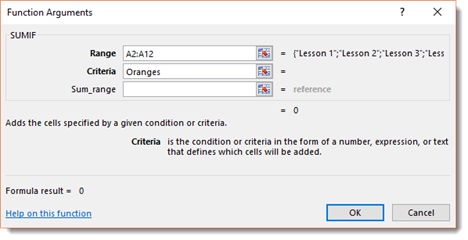
Enter the range you want to use for the criteria in the first range field. This will be the types of fruit.
In the criteria field, enter your criteria. We want the sum of oranges sold.
In the Sum Range field, enter the range you want to use to produce the sum.
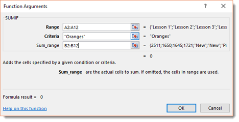
Click OK.
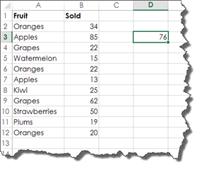
You can see the results in the selected cell.
The formula in the Formula Bar looks like this:
The COUNTIF Function
The COUNTIF function works much the same way as the SUMIF function, except that we are going to count instead of add. In addition, the COUNTIF function only has one range: the counting range.
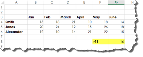
Using our worksheet again, we are going to count how many sales are over 11.
To do this, click on the cell where you want the results to appear.
Go to the Formulas tab, click the More Functions button. Go to Statistical, then select COUNTIF.
You will then see the Function Arguments dialogue box.
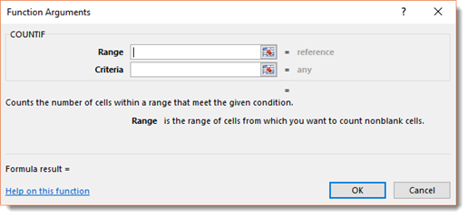
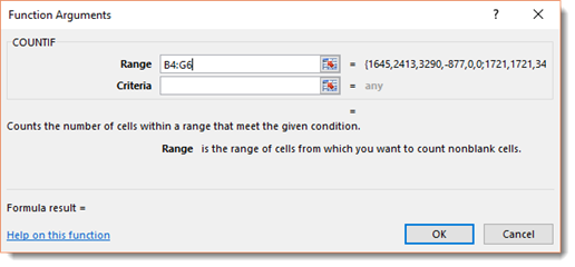
Enter the range of cells that you want to use to count.
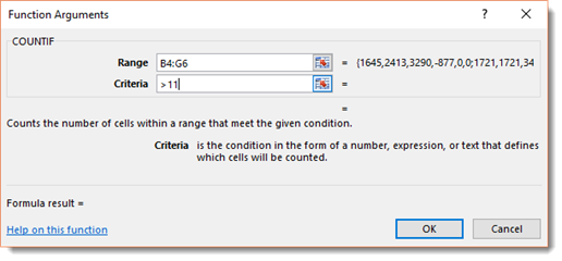
Now enter the criteria.
Click OK.
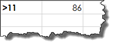
We highlighted our results below. We have 16 cells that are greater than 11 � or sixteen sales greater than 11.
The AVERAGEIF Function
The AVERAGEIF function will give you the mean of a selected range of cells based on criteria that you specify.
Take a look at our worksheet below.
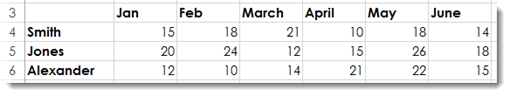
Let's say that we want to find the average for all sales over 11.
To do this, we would first select the cell where we want the results to appear.
Next, go to the Formulas tab. Click the More Functions button, then go to Statistical>AVERAGEIF.
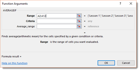
You will then see the Function Argument dialogue box, as pictured below.
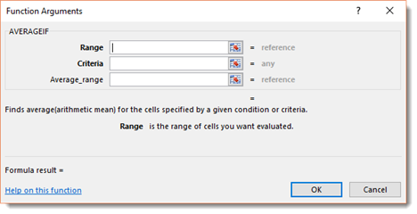
Notice that this dialogue box has two ranges just as SUMIF did. These two ranges will be used the exact same way, except we are wanting to produce the mean instead of the sum.
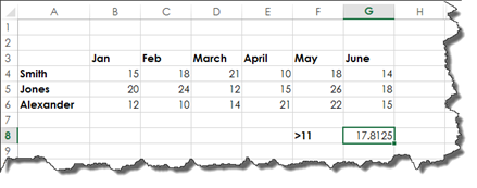
First, we are going to do a simple formula using AVERAGEIF.
We are going to enter the range of cells.

Then the criteria. Ours is >11.
Click OK.
Now let's use both ranges in the dialogue box.
Using the worksheet below, we want to figure out the average number of oranges sold.
First, we are going to enter the range to use for the criteria. This is the fruit column because we want to average the number of oranges.
Next, we are going to enter our criteria. Our criteria is Oranges because we want to average the number of oranges that were sold.
Then we want to enter the range to be used to figure out the average. That range is the cells that contain the number of fruit sold.
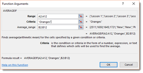
Click OK.
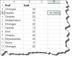
You can see the answer in the cell we have selected. If you check it with a calculator, this is indeed the average number of oranges sold.
Using Multiple Criteria with SUMIF, COUNTIF, and AVERAGEIF Functions
We can also use multiple criteria with SUMIF, COUNTIF, and AVERAGEIF functions.
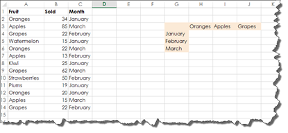
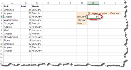
We can use our data on the left below to create the data on the right.
We can figure out the sum of oranges sold in January, for example.
When you use a SUMIF, COUNTIF, or AVERAGEIF function with multiple criteria, the function that you use will be a little different. Instead of =SUMIF you will use =SUMIFS. Notice the "S" on the end. The same holds true for COUNTIF. It becomes COUNTIFS. AVERAGEIF becomes AVERAGEIFS.
Let's use the SUMIFS function.
Select the cell where your results will appear.
Go to the Formulas Bar, then Math & Trig>SUMIFS.
You will then see the Function Arguments dialogue box.
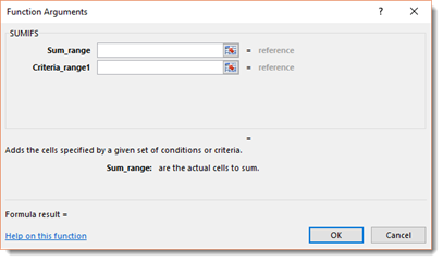
Enter the range to use to produce the sum.
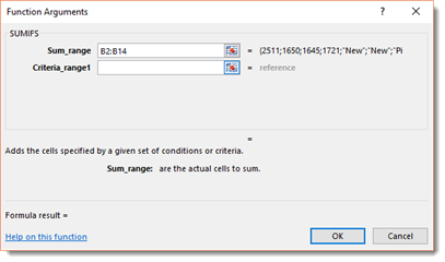
Now, enter the criteria range. This is the cells with months in them since our first criteria is January (since we want to figure out the number of oranges sold in January).
In the next field, we enter the criteria, which is January.
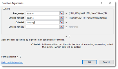
Now we enter our second criteria range, which is the cells with fruit in them. Our criteria is oranges, as shown below.
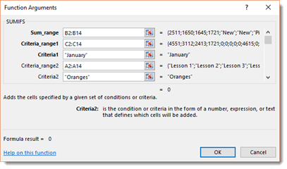
If we wanted, we could add more criteria ranges and criteria. When you are finished, click OK.
We can see the sum entered into our cell for us.
Our formula in the Formula Bar looks like this: