Linking two worksheets together means using references to cells in an external worksheet to bring data into your worksheet. Consolidating means to combine or summarize data from two or more worksheets.  The worksheets do not have to be in the same workbook. In this article, we are going to learn how to link and consolidate worksheets.

About Linking Worksheets

Whenever you link workbooks, you make it so that one workbook is dependent on the other. The dependent workbook is the workbook that contains the formula that links it to the other workbook. It is dependent on the information in the other workbook. The source workbook contains the information used in the dependent workbook. If the information linked to in the source workbook is updated or changed, those updates or changes will be reflected in the dependent workbook as well.

External Reference Formulas

To link one workbook to another, you will use an external reference formula. The syntax for this formula is = (WorkbookName) SheetName!CellAddress.

To create the external reference formula, open up the source workbook, then click the cell in the dependent workbook where you will put the formula.

Enter an equal sign into the cell to start the formula.  

Now go to the source workbook again. Select the cell or range, then press the Enter key on the keyboard.   When you select the cell or range, Excel creates the external reference, as shown below.

As you can see, the source workbook is Book1.xlsx. The worksheet is named Correctly Structured Data. The cell with the data we are linking to is cell A2.   The formula pictured above appears in the cell in the dependent workbook.

Linking to Unsaved Workbooks

You can also link to unsaved workbooks. Let's say you have two workbooks open that you have not yet saved. When you save the workbook that contain the external reference link, you will see the following dialogue box:

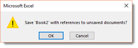
You can click the OK button; however, it is always best to save the source workbook first.

Opening Dependent Workbooks

When you open a workbook that contains external reference links, you will see a dialogue box that that asks what you want to do next.

You can:

• Update to update the data to the current data in the source file.

• Don't Update and use the values already in the dependent workbook.

• Help if you need to read more about links.

• Continue opens the workbook, but does not update the links.

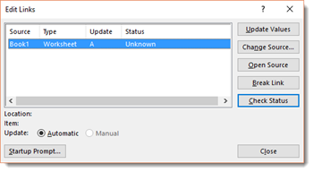
• Edit Links. If you choose Edit Links, you will see the Edit Links dialogue box. You can click the Source button to link to a different workbook. You can also click the Break Link button to destroy the link. You will keep the current values when you do this.

The Edit Links dialogue box is pictured below. You can also reach this dialogue box by going to the Data tab, going to the Connections group, then clicking Edit Links.

The Startup Prompt

If you open a workbook that contains several external reference links, you will see the Startup Prompt dialogue box.

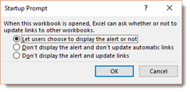
You can also reach this dialogue box by going to the Edit Links dialogue box, then click the Startup Prompt button.

In the Startup Prompt dialogue box, you can specify how Excel will handle the links when the workbook is opened.

Updating a Link

To make sure that you have the current data from the source workbook, you can update the link.   To update the link, go to the Edit Links dialogue box.

Click on the source workbook, then click the Update Values dialogue box.

Changing the Source Workbook

If you need to change the source workbook, go to the Edit Links dialogue box. Click on the source workbook that you want to change, then click the Change Source button.

You will then see the following dialogue box:

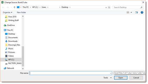
Select a new source file, then click the Open button.

Destroying Links

If you want to remove links to a source workbook and turn the external reference formulas to values, go to the Edit Links dialogue box. Click on the Break Link button.

Consolidating Worksheets

You can consolidate two worksheets from the same workbook, or you can consolidate several workbook files. You don't always have to create link formulas to consolidate worksheets, but there are certain circumstances where you will have to do just that. 

Consolidating worksheets or workbooks can be easy if the information is the same. For example, if you have two worksheets that contain sales data, and they both have the same column headers. However, consolidation can be more difficult if they do not contain the same information.   That is okay, though. We will teach you all you need to know in this article.

Consolidating Using Formulas

When you consolidate using formulas, you create formulas that reference other worksheets or workbooks.   This means if the information in one worksheet or workbook changes, the formulas are updated automatically.   That is a huge benefit to using formulas to consolidate worksheets or workbooks. 

The standard formula to consolidate worksheets in the same workbook is: =SUM(Sheet2:Sheet10!A1).

This formula will find the total for cell A1 in the worksheets named Sheet 2 through Sheet 10. 

If you want to consolidate information from other workbooks, you would use an external reference formula. Here is an example: =[Workbook1.xlsx]Sheet1!B2+[Workbook2.xlsx]Sheet1:B2

This formula adds the values in cell A1 from the Sheet1 of two workbooks. 

If the worksheets are not structured the same, you can still use formulas; however, make sure that each formula refers to the proper cell.

The Consolidate Dialogue Box

Arguably, the best way to consolidate worksheets is to use the Consolidate dialogue box. If your worksheets are not structured the same, this may be the best route to go. You can use the Consolidate dialogue box to consolidate worksheets in the same workbook – or in different workbooks. In addition, you can use the dialogue box to create consolidations that are static, which means no link formula, or dynamic. Dynamic consolidations contain link formulas.

The consolidation feature in Excel uses two methods of consolidation:

1.       By position. Choose this if your worksheets are structured the same.

2.       By category. Rows and columns are what Excel uses to match data in source worksheets.   If the data is structured differently or is missing rows and columns, use this consolidation method.

To open the Consolidate dialogue box, go to the Data tab. Click on Consolidate in the Data Tools group.

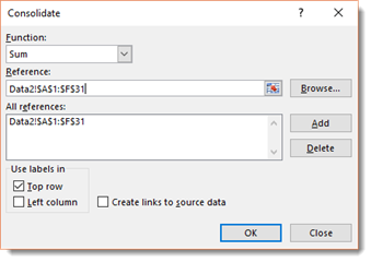
The Consolidate dialogue box is pictured below.

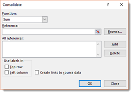
Let's talk about the options in the Consolidate dialogue box.

The Function dropdown list asks for the type of consolidation you want to use. SUM is the common type.

The Reference field allows you to specify a range from the source file that you want to consolidate with your worksheet. You can enter the range yourself, or select it from the source file. You can also use named ranges if you want. After you enter the range, click the Add button so it gets added to the All References section of the dialogue box.

The All References field contains the list of references you have added.

The Use Labels In section lets you decide if you want to consolidate by using labels in the top row or left column – or even both. If you are consolidating by category, make sure you select an option.

Put a checkmark beside Create Links to Source Data if you want to use summary formulas for each label. Excel will also create an outline when you select this option. If you leave the box empty, the consolidation will not use formulas.

The Browse button opens another dialogue box from which you can select another workbook to open. The filename will be put in the Reference box. You will just have to supply the range. 

The Add button lets you add references to the Reference box.

The Delete button lets you delete a reference from the All References list.

Consolidating Worksheets: An Example

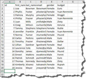
Let's show you how easy a consolidation can be by doing an easier consolidation as an example.   For this example, we are going to use two worksheets in the same workbook.   They both contain the same structure and the same types of data. In other words, they have the same column headers and the same types of information in the rows. Our worksheets are named Data1 and Data2.   We are going to consolidate the information in sheet Data1.

To start with, we are going to click the cell in Data1 where we want the information from Data2 to begin. 

Next, we are going to open the Consolidate dialogue box by going to the Data tab, then clicking the Consolidate button as we learned to do in the last section of this article.

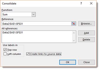
The Consolidate dialogue box is pictured below:

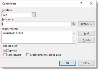
As you can see, we chose SUM from the Function dropdown menu.   This will allow us to combine the data.

Next, we are going to click in the Reference field. Since we are consolidating worksheets from the same workbook, we are going to then click in the second worksheet – or Data2 – and click and drag over the data we want to consolidate with the first worksheet – or Data1.

Click the Add button if the range does not appear in the All References field.

Next, we chose to use the labels in our top row, since these are the column headers. 

We are also going place a checkmark beside Create Links to Source Data.  This is not necessary since the worksheets are in the same workbook.  We are doing it because if the information in sheet Data2 changes or is updated, we want it to be automatically updated in the sheet Data1.

You may use Excel 2016 to store data in spreadsheets. The data may represent sales records, expenses, invoices, loans, or any number of things.   The data that you use in your spreadsheets could come from any number of sources, such as websites and text files.   While you could take the time to transcribe the data into Excel, that would be very time consuming. Instead, Excel gives you several methods to import different types of files that contain your data.

File Types That Can Be Imported Into Excel 2016

Excel 2016 can import any number of file formats.  Let's take a look at the various formats you can import with Excel 2016.

Excel formats. Excel can import other spreadsheet file formats, such as XLSX, XLSM, XLSB, XLTX, XLTM, and XLAM.   These are current spreadsheet file formations. In addition, Excel 2016 can also import files from older versions of Excel. These formats include XLS (Excel 4, 95, 97, 2000, 2002, and 2003), XLM (Excel 4 macros), XLT (Excel template), and XLA (Excel add-in). 

Database formats. Excel 2016 can also import the database file formats .mdb and accdb from Microsoft Access, as well as dBase files from dBase III and dBase IV.   You can perform a query on a database so that you only import the records that you need.

Text File Formats. A text file does not contain formatting. Excel can open CSV, TXT, PRN, DIF, and SYLK text files.

HTML files. Most basic HTML files will appear the same way as they do in the browser. However, if the file uses CSS, or Cascading Style Sheets, it may not look the same at all.

XML files. Simple XML files will display without a problem. More complex files might be a little more difficult. If you have trouble importing XML files, the easiest thing to do is use the Tell Me tool in Excel.

Importing Files into Excel

To import files into Excel 2016, go to Data tab, then the Get External Data group. 

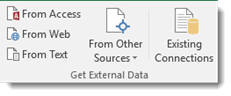
Select from where you want to import data. As you can see in the snapshot above, you can select From Access, From Web, or From Text. You can also click the From Other Sources dropdown arrow.

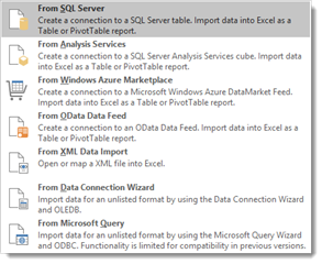
Let's choose From Text.

When you click on From Text, you will see the Import Text File dialogue box, as shown below.

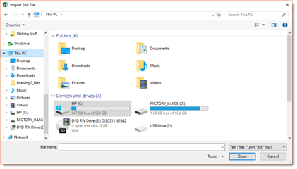
We are going to import a plain text file – or .txt.

Once you select the file, then click the Open button, you will see the Import Wizard dialogue box.

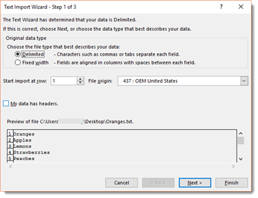
In the dialogue box above, you can see a preview of the file. In the preview, the rows are labeled.   Above the preview, you can specify the row in which you want to start the import. For example, you may want to start at Row 3.

Click the Next button.

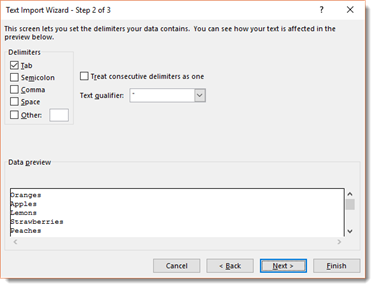
Set your delimiters.   You can choose different delimiters to see how it affects the text.  

Click the Next button.

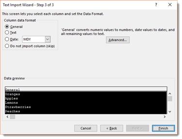
Select a format for the column that will contain the data. General is selected by default. We are going to change this to Text for our data.

Click the Finish button.

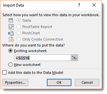
Next, select how you want to view the data, as well as where you want to place it. We have chosen to import our data into a new worksheet. 

However, you can also choose to place it into an existing worksheet by specifying the cell where the data will begin to be inserted.   This is how you import a text file into a specified range in a worksheet.

Click the OK button when you are finished.

Our data from a plain text file is now imported into Excel.

Copying and Pasting Data

It goes without saying that you can also copy data from one source, such as a text file, and paste it into your worksheet. You will probably have to clean up the data after you paste it, but it can seem like a shortcut if you do not want to use the built-in tools that Excel provides for importing data.

Cleaning Imported Data

Once you import data into a worksheet, you may have to clean it up so it appears as you need it. This may include removing duplicate rows, converting text in cells into different columns, and filling in gaps.   For the rest of this article, we will cover data cleanup techniques in Excel 2016.   Some we will teach you.  

Cleaning Up Duplicate Rows

When you import data into Excel, especially if you import into an existing worksheet, you may have duplicate rows. Duplicate rows contain the same data. We do not want duplicate data in our worksheet. We want to clean that up.

To do this, click on any cell in your data range.

Next, go to the Data tab, then Remove Duplicates in the Data Tools group.

You will then see the Remove Duplicates dialogue box, as shown below.

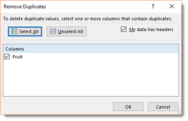
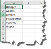
Put a checkmark before the columns you want to search.   We are going to search for duplicate data that exists in rows below the Fruit column.

Click the OK button.

Excel 2016 removes the duplicate data for you.   You do not get to pick and choose if you want to keep some of the duplicate data. Excel 2016 removes all duplicates.

Finding Duplicate Rows

There may be times when you want to keep some of the duplicate rows.   Perhaps some of the duplicates are needed in your data.   If you want to find the duplicate rows on your own so you can choose what to do with them, you will use a formula.

Let's say you want to find duplicate rows in columns A through C.

Enter this formula into cell D2.

In cell E2, were are going to use the COUNTIF function.

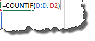
Copy these formulas down all of your rows.

Column E displays the number of occurrences in the row.

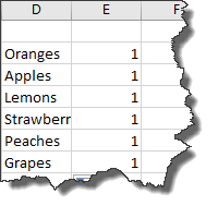
Since there is only one occurrence, we know we do not have any duplicate data. If it showed more than one occurrence, we would know there was duplicate data. At that point, we could decide what to do with it.

Splitting Text

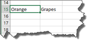
Take a look at the snapshot below. As you can see, we have two words in one cell.

Sometimes when you import data, this might happen. Text data that should appear in two columns appears in one instead.

To fix this, first make sure that there are enough empty columns to the right to be able to successfully split up the text data.  

Make sure the data is selected, then go to the Data tab. Choose Text to Columns in the Data Tools group.

You will then see the Convert Text to Columns Wizard.

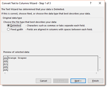
Choose if the data to be split is delimited or fixed width. Delimited means the data you want to split has delimiters. A delimiter might be a comma, slash, or space.   Fixed width means each piece of data has the same amount of characters. 

We are going to choose Delimited.

Click the Next button. 

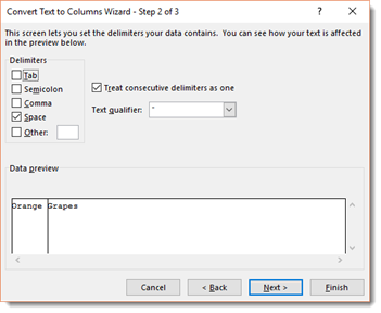
In the next window of the wizard, pictured above, we are asked to specify our delimiter. Our delimiter is a space. In the Data Preview section, you can see where the column break will be placed.

Click the Next button.

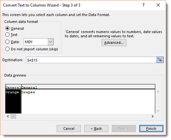
Now you get to select the formatting for the cells that your data occupies.   You can see in the Data Preview section which column you are formatting. You can click on the other column to select it. 

We want both columns to be in text format.

Click the Finish button when you have chosen the formatting.

As you can see in the snapshot below, our text data now appears in two columns.

Changing the Case of Text Data

Let's say we want to change our data to all uppercase.   Or perhaps we want to change it all lower case. The text data below is in Proper Case, but we can change it to uppercase or lower case easily enough by using functions. 

To change it to uppercase, use the UPPER function.

To change it to lower case, you the LOWER function.

To change it back to Proper Case, use the PROPER function.

Removing Strange Characters in Imported Data

Have you ever had strange characters appear in your data?   There is no doubt you have had it happen before. Perhaps you have saved an email, only to open it later and have it full of strange characters that seem like gibberish.    This can also happen when you import data.

To remove strange characters in your data, click on the offending cell, then enter the formula =CLEAN(B2). Of course, you would enter the coordinates of your offending cell.

Joining Columns

We learned how to separate data into two columns, but what if you want to join data from two columns? Let's say you want to join the data in columns A, B, and C.  

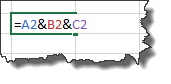
To do this, you would use this formula: =A1&B1&C1

If you need to insert spaces between the cells so the data does not all combine together, you would use the formula: =A1&" "&B1&" "&C1

Rearranging Columns

If you need to rearrange the columns in a worksheet, click the header of the column you want to move, then go to the Home tab. Click Cut in the clipboard group.  

Next, click on the column to the right of where you want to place the column. This selects the column. Now right click your mouse, then select Insert Cut Cells from the context menu.

Filling in Gaps in Imported Data

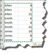
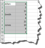
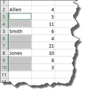
When you import data into Excel, sometimes you can have gaps in your data.   Gaps are rows where data should appear, but it does not. Take a look at the snapshot below to see what we mean.

We would want the names Allen, Smith, and Jones to appear in the beginning of any row that contains data related to them.   Instead, when we imported data, it only put the name before the first row of data that related to each person.

To fix this, start out by selecting the range of data that contains the gaps, as we have in the snapshot below.

Next, go to the Home tab, then the Editing group.   Click the Find & Select dropdown arrow, then choose Go to Special.

You will then see the Go To Special dialogue box.

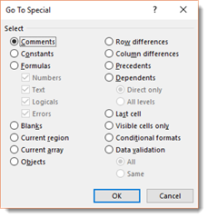
Select Blanks, then click the OK button.

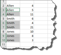
As you can see in the snapshot below, doing this selects the blank cells in the range.

Now type in the Formula Bar. Type an equal sign (=) and then the coordinates of the first cell in the range. 

Instead of pressing ENTER as you normally would, press CTRL+ENTER.

Select the range of cells again, then press CTRL+C to copy.   Next, go to the Home tab, then the Clipboard group. Click the Paste dropdown and select Paste Values to convert formula to values.