
Formulas Using Internal Functions
In each calculation, the equal sign is the first character in a cell's text. The equal sign tells Excel that text is in the form of a calculation, and the values stored are mathematical equations. The following is a simple calculation:
=A1+B1
The above formula tells Excel to add the values in A1 and B1. Values can be literals instead of references:
=1+3
This formula adds the numbers one and three and displays the result in the selected cell.
Excel has several functions that perform a vast array of mathematical actions. Suppose that you want to add values in A1 through D1. You could reference all four cells, but this takes time and isn't feasible if the range of cells expands from four to 100 columns. Instead of typing each cell one-by-one, Excel has the method SUM that you can use.
Type the following values in cells A1, B1, C1, and D1 respectively:
3
10
4
7
Using the SUM function, you can add these values using a formula. Type the following formula in cell D3:
=SUM(A1:D1)
Notice that a range is used, so you don't need to specify each cell individually. The SUM function is an internal method available in Excel, so you don't need to specify the action to take on values either.
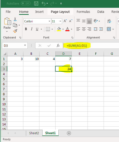
(Using the SUM function)
Just like any other formula, the result is displayed in the cell that contains the formula. Excel has several internal functions that provide easy access to calculations and results.
Another common function is AVERAGE. You could add up each value in a range of cells, then divide by the number of values but you'd need to manually count the number of cells in your range. If data changes and you add more values to your range, you'd need to re-count the number of values again. The easier way to calculate the average in a range of cells is to use the AVERAGE function.
Change the formula in D3 to the following:
=AVERAGE(A1:D1)
The result changes and displays in the active cell.
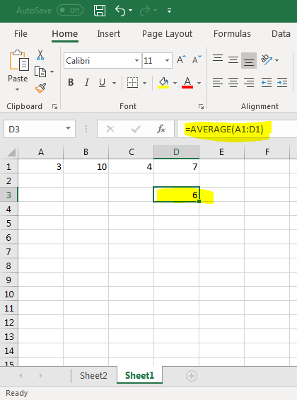
(Formula using the AVERAGE function)
Notice that the syntax is the same, but the function used is the same. Each function has its own parameter syntax.
Functions that perform basic calculations aren't limited to just one range of cells. These functions can take several ranges and perform a calculation. Each range is separated by a comma. We can use the AVERAGE function again to illustrate.
Change the current formula in D3 to the following:
=AVERAGE(A1:D1,F1:G1)
Add the values "5" and "6" respectively in cells F1 and G1. Without these values, Excel uses the default value "0" in empty cells for numerical calculations.
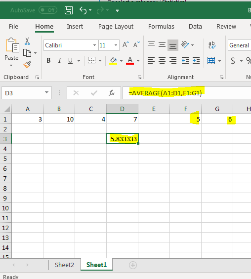
(The AVERAGE function with multiple ranges)
Using commas, you can add as many ranges as you need in an Excel function provided it's mathematically feasible and the function allows it. In the image above, the new range is added separated by a comma and Excel automatically updates the results.
Finding a Function's Parameters
Excel has dozens of functions to choose from, and even if you remember the function's name it's difficult to remember each one's parameter requirements. If you use the wrong number of parameters or set up a function incorrectly, Excel displays an error on your worksheet. To avoid these issues, you can use Excel's function lookup feature to find the function that does the calculation that you need and the parameters that must be passed to the internal process.
The function lookup button is directly left of the input text box where you enter content.
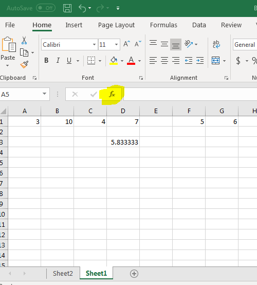
(Function lookup button)
Click the button to open a new popup window.
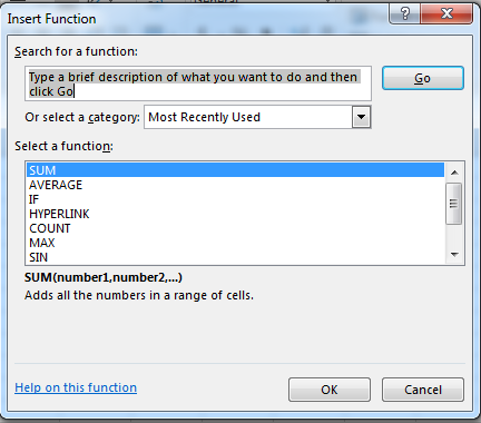
(Function lookup window)
The first section of the popup window tells you to enter a description to find a function. Excel attempts to find a function based on your input. Also notice the dropdown box under the search text box. The default selection lists the functions used the most often, so the functions you see immediately are the ones that you use most often. Since we used SUM and AVERAGE in previous examples, Excel displays these two functions at the top.
If the search text doesn't find any appropriate function, you can search through each category. Click the category dropdown, and you'll see a long list of options. These categories will narrow down your search and help you find an appropriate function.
The third important part of this window is the text under the list of functions. This is where you find the syntax that you must follow when you use it in your spreadsheets. In the image above, the SUM function is highlighted. Below the list of categories, you can see the syntax required. SUM takes a range of numbers, a single cell reference, or several ranges and numbers separated by commas.
Under the parameter syntax is a small description that explains the function's action. If you didn't know what happens when SUM is included in a formula, you can read this description to get a better understanding. Many of the functions in Excel are specific to an industry, so you'll need this description to understand a function's features.
Let's take a random action and search for the best function available. Suppose you want to round a number. Unless you know the function by memory, you must search Excel's list of categories and available functions.
Type "round" in the search text box.
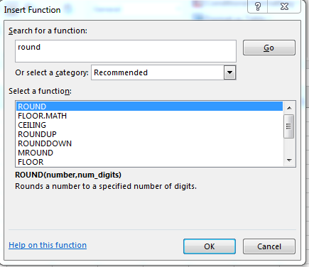
(Searching for functions that round numbers)
Click "Go" after you type your search phrase, and if Excel finds any recommended functions it will show them in the list. The first result is the ROUND function. Click it and notice that the parameters and a brief description are shown below the list of recommended functions.
Click on CEILING. Another description with a list of parameters displays. CEILING takes different parameters rounding up to the number of significant figures (decimal points) specified. For a simple rounding function, the best fit seems to be the ROUND function. You can click through the other functions to determine if any others fit your search query. Some functions that display are specific to industries listed in the category dropdown.
Using Functions from Search Results
After you find the function that you want to use, Excel helps you implement it. It's a helpful feature when you're unsure how to work with specific parameters.
The AVERAGE function calculated to "5.833333" displayed in cell D3. We can round that number using the ROUND function. You can embed several functions in one cell's calculation as long as syntax is properly typed. Since we want to round the number from the AVERAGE function, it should be one of the parameters in the ROUND function.
Change the content entered into D3 to the following formula:
=ROUND(AVERAGE(A1:D1,F1:G1), 2)
The ROUND function takes two parameters, and one of these parameters is the AVERAGE function results. After the AVERAGE function, a comma and value of 2 are the second part of the function. The "2" value tells ROUND that you want to round to the second decimal point.
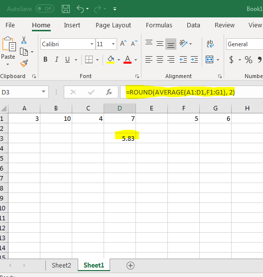
(Embedded functions ROUND and AVERAGE)
In many occasions, you won't know what to use in function parameters and Excel can help you work with functions that you're unfamiliar with. Click the F3 cell to use a new one instead of overwriting the current cell with the AVERAGE and ROUND functions.
In this example, we want to know the number of cells in a selected range. When you have only a few cells in a range, it's easy to do a quick check and count the number of cells in a range. However, when you work with large spreadsheets with ranges that span thousands of cells, it's nearly impossible to accurately count the number of cells in a range. Excel provides the COUNT function that counts the range for you, so you don't need to tediously go through each of your number ranges.
After selecting the D3 cell, click the function button. The function search window opens again. You can type "count" in the search text box, or COUNT could be shown in the most recently used by default. Click "COUNT" to select it from the list of results and then click "OK" to open another window with a list of parameters.
Using this feature, Excel guides you through parameters for the selected functions and helps you choose cells to add to parameters.
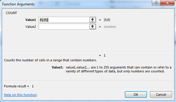
(Parameter selection for the COUNT function)
Notice that the value selected is described below the list of parameter selections. This description helps understand the cells that you should include in the function's parameter. In the image above, the first value is automatically entered. You can see a preview of numbers on the right side of the value text box. Change this range to "A1:D1" and click "OK."
The result displays in the F3 cell. Notice that the result displayed in the F3 cell is "4," which is the number of cells represented in the COUNT range. This test shows you that COUNT is working properly, so you can use it in larger ranges and trust that you're using it properly. Remember that you aren't limited to just one range. Because you've viewed the parameters from the function search window, you know that you can use an additional range by separating it with a comma or using the function arguments help window to select each range using a mouse.
Working with formulas is one of the more difficult parts of working with Excel. Some formulas can be complex and require several lines of Excel code. If any one mistake is made, your formula will return an error and you must find the mistake or this error displays on your spreadsheet. A combination of typing syntax in Excel and using the function search feature will help you build these formulas without memorizing a long list of parameters and save you the time of building results from mathematical equations.
Mathematical Operators
The main ingredient in any formula � aside from the numbers � are the mathematical operators. These operators tell Excel how to calculate a formula.
That said, let's start out with a simple formula, learn how to enter it into Excel, and learn the operators.
The formula we're going to use is:

Now, in the formula above, we want Excel to tell us the sum of 5+2. The numbers 5 and 2 in this equation are called operands. Operands in Excel can be either a number or a cell.
For instance, if we wanted to add the value of two cells, say D1 and D2, we'd write:

When we use a cell name instead of a number, it is called a reference.
The + symbol is called an operator. You use operators to tell Excel what kind of calculation you want it to perform. In this case, we want to add the two numbers together to find the sum.
Excel recognizes four different kinds of calculation operators. They are:
Arithmetic operators--used to perform basic mathematical operations such as adding, subtracting, multiplying, and dividing.
Comparison operators--used to compare values.
Text operators--used to join two distinct text strings into a single string. For instance, "global" & "warming."
Reference operators--used to combine ranges of cells for calculations
The table below contains a list of recognized operators.
|
Operator |
Meaning |
|
Arithmetic operators |
|
|
+ |
Addition |
|
- |
Subtraction |
|
* |
Multiplication |
|
/ |
Division |
|
% |
Percent |
|
^ |
Exponentiation |
|
|
|
|
Comparison operators |
|
|
= |
Equal to |
|
> |
Greater than |
|
< |
Less than |
|
> = |
Greater than or equal to |
|
< = |
Less than or equal to |
|
< > |
Not equal to |
|
Text operator |
|
|
& |
Connects two values to produce one continuous text value |
|
Reference operators |
|
|
: |
Range operator |
|
, |
Union operator, combines multiple references into one reference. |
|
(space) |
Intersection operator |
Creating a Formula
In the last section, we learned to create a simple formula. Let's continue with constructing formulas.
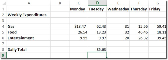
Now let's say we wanted to create a weekly expense report in Excel.
We stopped for gas twice on Tuesday and have two receipts, one for $29.92 and the other for $32.51. We'd click on the correct cell (in this case D4) and type =29.92+32.51. Remember, a formula always begins with an equal (=) sign.
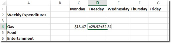
The equation appears in the formula bar as well as in the individual cell as you type it. Hit Enter and the equation disappears, leaving only the sum of the two numbers:
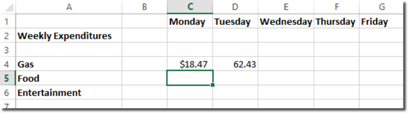
If you want to see the formula again, click on the cell. The formula will be visible in the formula bar.
You can also perform a calculation based on the values within a series of cells. Let's add up the figures in column D. The individual cell coordinates are D4, D5, and D6. We want the total to appear in cell D8, in the row called Daily Total. Select that cell (D8) and verify your selection by checking the Name Box.
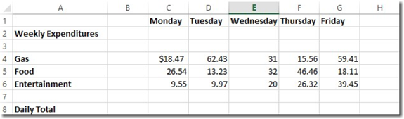
Now we'll type =SUM(D4:D6) in Cell D8. The equals sign tells Excel that you are going to enter a formula. The SUM tells it to add the following numbers and the colon tells it the range (D4 to D6).
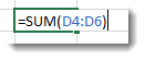
You'll notice the cell references appear in blue. Also, the cells that you reference become shaded blue as well. This gives you a visual representation of the selected range.
Hit Enter and the sum will appear in cell D8.
Because the sum depends upon the numbers in cells D4 thru D6, Excel will automatically recalculate the sum whenever the values of those cells change.
Order of Operation
When constructing a formula, it's important to remember that Excel reads formulas from left to right using the natural order of arithmetic operation. In other words, Excel multiplies and divides before it adds and subtracts.
If you want it to add or subtract before it multiplies and divides, or you want two numbers multiplied first, then you must use parentheses. Look at the example below:
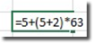
In this formula, Excel 2019 will first add 5+2 since they're in parentheses. Next, it will multiply that answer times 63. Finally, it will add five.
The answer is:

This is the correct order. If you wouldn't have added the parentheses, the answer would have been 136. Here's why. Excel would have multiplied 2*63, then added five, then added five more. Make sure that you "talk" to Excel by adding parentheses when needed.
Editing a Formula
You can edit a formula by clicking on the cell and editing the formula in the Formula Bar.
Here's our formula as shown in the formula bar:

We changed 63 to 65 in the Formula Bar, then hit Enter.
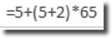
The calculation is automatically changed in the cell:

Formula Errors
Sometimes when you type a formula in, instead of Excel calculating and providing you with the answer, you'll get an error message such as #NAME?
When this happens, Excel is letting you know that some element of the formula or the cell in the formula is stopping Excel from doing its calculation. These types of error messages are called error values.
When you see an error value appear, you must figure out what caused it, then edit the formula to fix the problem.
|
Error Message |
What It Means |
|
#DIV/0! |
This is the error value shown when a formula requires division by a cell that contains the value 0 or is empty. |
|
#NAME? |
This appears when a formula refers to a range name that doesn't exist. (D15:D22) It can also appear when you don't put quotation marks around text used in a formula because Excel will think the text is a range name. |
|
#NULL! |
This appears when you insert a space instead of a comma to separate cell references that are used for arguments in functions. |
|
#NUM! |
This appears if Excel finds a problem with a number in formula, such as a wrong argument in a function or calculation that creates a number too large or small to be represented. |
|
#REF! |
This appears when Excel finds an invalid cell reference. If you delete a cell that's referenced in a formula, you might see this message |
|
#VALUE! |
This appears when you enter in the wrong type of argument or operator in a function. It can also appear when you enter a mathematical operation for a cell that contains text. |
AutoSum
PCMag.com defines the AutoSum as a "function in a spreadsheet program that inserts a formula in the selected cell that adds the numbers in the column above it."
In other words, if we select cell E13 in the worksheet below, the AutoSum feature will add the numbers in the cells above it that are still in the same column.
To use AutoSum in Excel, go to the Editing group under the Home tab on the Ribbon.
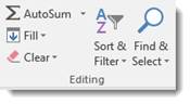
As you can see, you can use this tool to calculate the SUM, AVERAGE, COUNT, MAX, or MIN.
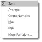
- SUM is the sum of the values.
- AVERAGE is the average of all the values in the cells.
- COUNT counts the number of cells that contain numbers.
- MAX is the largest value.
- MIN is the smallest value
It can also select the most likely range of cells in a column or row that you want to use as the argument, then enters them for you.
You don't have to do anything to use the SUM feature of AutoSum but select the cell. If you want to use AVERAGE, COUNT, MAX, or MIN, you need to select them from the dropdown menu pictured above.
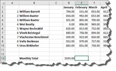
Let's calculate the sales total for column E in our worksheet.

As you can see, we selected cell E13 in our worksheet. This is where the sales total will appear.
To add the sum of all the values above cell E13, we go to the Home tab, then click the AutoSum button.
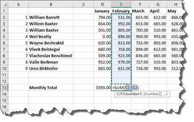
Excel 2019 automatically selected the range of cells we want to use in the argument, then entered the arguments into our function.
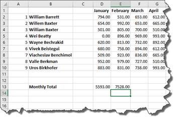
Hit Enter.
The total appears in cell E13.
If you want to edit the argument before pushing Enter, you can do that.
Locating the Function You Need
Finding the function you need can seem a daunting task. Of course, you can insert a function by using the Ribbon or Formula Bar, but you can also go to the Function Library under the Formulas tab.
In the Function Library, functions are broken down into categories.
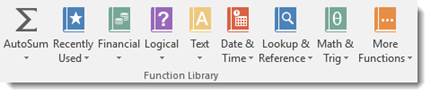
Let's say we want to look for a function in Lookup & Reference.
Click the downward arrow. You'll see all the functions that you can use under this category.
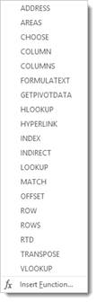
You can click on any one of the functions, and the arguments dialogue box will appear so you can enter your arguments.
You can also click Insert Function at the bottom of the dropdown menu.
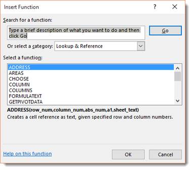
All the Lookup & Reference functions are displayed. Choose the one you want, and click OK.
References
A reference simply tells Excel where to find the information you want to use in a formula. As you've already learned, by default Excel 2019 uses the A1 reference style, or coordinate system, to identify cells. You can use these coordinates for references or you can use labels and names.
Using labels and names makes it easier to understand the information you are entering into the formula. For instance, the formula "=SUM(WednesdayTotal)" is easier to understand than "=SUM(E4:E6)
Using Names as References
As you learned earlier, a label is used to identify a range of cells such as a column or a row. You can also create a name to represent a cell or a range of cells for quicker reference in a formula. Names can also represent an unchanging number (called a constant) or even a formula.
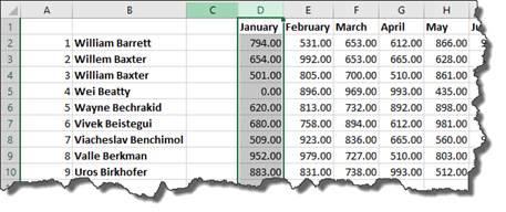
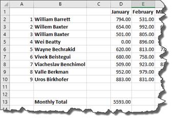
In the snapshot below, we want to name the column January as "January." This way, when constructing formulas, we can simply enter in January instead of a range of cells.
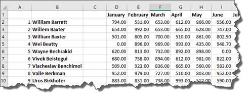
To do this, we're going to select the column "January".
Next, we go to Formulas tab, then the Defined Names group.
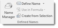
Click the dropdown arrow beside the Define Name button.
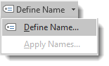
Select Define Name.
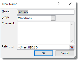
We want the name to stay the same as our label January. If we didn't, we'd enter a new name in the Name field, then the scope -- if we want it to apply to the entire workbook or just the worksheet -- then any comments we want to add.
Click OK.
Now we've named this column.
Instead of having to write out the formula as =SUM(D2:D10), we can simply enter in =SUM(January), then hit Enter. The calculation appears in the cell.
Now let's create a name for a constant. In this example, we'll say it's sales tax.
Click in an empty cell, then go to Define Name.
Give it the Name: SalesTax.
The scope is the workbook.
In the Refers To section, we want to enter .08.
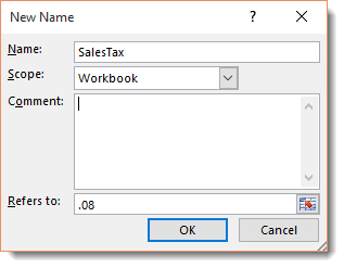
Click OK.
To see all the names you've created if you need a reminder, click the Names Manager in the Defined Names group.
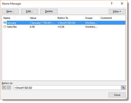
In the dialogue box above, you can add, edit, or delete names.
Now, let's go back to the SalesTax name for a minute. We now have a reference for sales tax. We can then use that reference in a formula. In the example below, we'll apply sales tax to the total for January, which is cell D13.
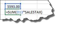
As you can see in the formula above, we entered the function SUM, then included the values used for the function in parentheses. These values were from D13 and the SALESTAX reference.
Hit Enter.
We now get the amount of sales tax.

We can now add (SUM) the amounts from D13 and D14 together to get a grand total.
Absolute, Relative, and Mixed Cell References
There are two kinds of cell references: Absolute and Relative.
A relative reference in a formula depends upon its position in a worksheet. For instance, the cell coordinates in the following example "B4:B6" are relative references.
In the example below, we can copy the formula in cell D13 and paste it as a formula into cell E14.
When we do this, the formula stays the same, but the relative references change.
We'll show you how to copy and paste formulas in just a minute.
For right now it's important to realize that the formula stayed the same, but the relative references changed because Excel recognized the relationship between the formula in cell D13 and its cell range (D2:D10). When we pasted the formula into a new cell, it created the same relationship in the new position.
That's a relative reference.
An Absolute Reference does not depend upon its position in a worksheet. For instance, if the value in cell D13 were an absolute reference, when we pasted the formula in cell E13, the formula would read: =SUM($D$2:$D$10).
The symbol "$" in cell coordinates tells Excel 2019 that this is an absolute reference. To create an absolute reference, type a dollar sign before the column reference and row reference in the formula.
A mixed reference contains both an absolute reference and a relative reference. Which means, it can either contain an absolute column and a relative row, or a relative column and an absolute row.
Copying and Pasting Formulas without Relative References
At some point when using Excel 2019, you may want to copy a formula, then paste it into a different cell, as we did in the last section.
Let's use the same example again.
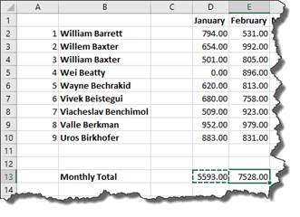
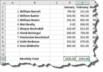
We want to use the same formula in cell E13 as we did in D13. This formula calculates sales totals by month.
To do this, we are going copy the formula in cell D13 and paste it as a formula into cell E13.

We start out by selecting cell D13, right clicking, then choosing Copy from the context menu.
Next, we click cell E13 to make it active, right click, then either click on the Formulas icon, as highlighted below.
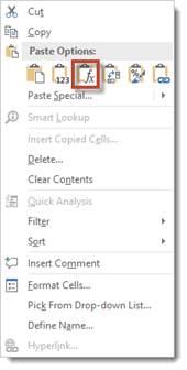
Or by clicking on the arrow beside Paste Special and selecting Paste Special.
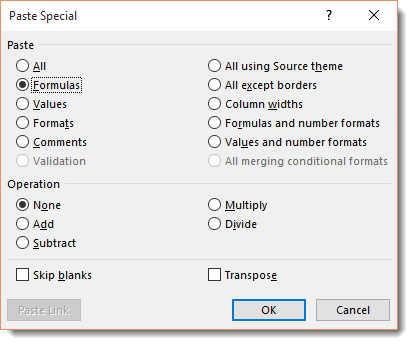
Select Formulas, then click OK.
As you can see below, the total for February then appears in cell E13.

The formula remained the same. Only the relative references changed when we pasted the formula into cell E13.
Now let's change it to absolute references.
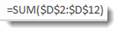
We don't want the references to column D to change, so we add a dollar sign before the column and row in cell D13.
Now, we can click on cell D13 in our worksheet. You can either click Copy under the Home tab in the Clipboard group, of you can right click and select Copy.
Now click on the cell that you want to paste into. For us, it's E13.
Right click and select Paste Special>Paste Special.
We want to paste the formula.
Click OK.
As you can see, our formula with our absolute values appear in cell E13.
If you don't add absolute values to your formula in the cut/copied cell, it will change the cell references to the pasted cells coordinates, as mentioned above.
Copying and Pasting Only Values from One Cell to Another
You can also simply paste the calculation and value from a formula in one cell into another.
Copy cell D13 again.
Next, go to cell E13 and right click, then choose Paste Special>Paste Special.
In the Paste Special dialogue box, check Values.
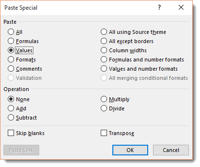
Click OK.
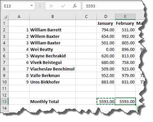
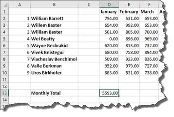
You can look in the Formula Bar with cell E13 selected and see that only the value was pasted, not the formula.
Linking Formulas
When you paste a formula, you may want to link back to the cell where you copied the formula. There may be data there that needs referenced, etc.
For example, you may have one table in a worksheet that lists your employee's sales figure by the month, then presents a grand total of sales by all employees for each month of the year.
However, you may also have another table in your worksheet that deducts total expenses for each month from the monthly sales figures in order to determine profit. You may want to use the formula you placed in a cell to calculate the grand total of sales for the month of January in the other table so you deduct expenses from that amount. The easiest way to do that is to link formulas.
To link formulas, first select the cell that contains the formula that you want to copy. In our example, it's cell D13 since that contains the sales total for January. We want to link to the formula instead of simply copying and pasting the formula or the calculation. We want to link to it so if the values change in the formula in cell D13, it will also change in our other table where we are using the formula.
We want to move the formula from D13 down further on our worksheet where we subtract expenses.
Here's where we subtract expenses in our worksheet:
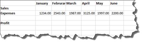
As you can see, we have the expenses entered for each month. Now all we need are the sales totals. We want to fill in January sales with the calculation from D13.
To do this, we start out by copying D13.
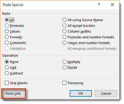
Next, we go to the cell in our other table that represents total sales for January. This is cell C22. Right click on it, and choose Paste Special>Paste Special.
Click the Paste Link button.
As you can see, the calculation is now pasted into cell C22.
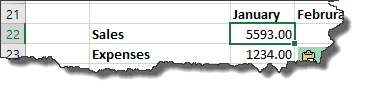
Now, if you look at the Formula Bar whenever you click on cell C22, you'll see it links you to cell D13.

Notice the references were changed to absolute.