The FIND Function

LOOKUP functions find content in a cell, but you use the FIND function to search for text within text. The FIND function is useful when you have a sentence or several terms within a cell, and you want to find a word or string of characters within this text.

The following is the syntax for the FIND function:

FIND (<text to find>, <search within this text>, [OPTIONAL]<character start>)

• Text to find: this is the text that you're searching for
• Search within this text: specifies the cell that contains the text
• Character start [OPTIONAL]: the character at which you want to start the search

Using the "Expense" report example, you could use the FIND function to identify a string within text. You might want to find cells that contain the word "payment" to identify if there was a payment made. You can do this with the FIND function to avoid lookups that require exact matches.

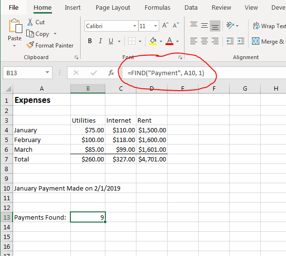
(FIND function example)

The return value for the FIND function is an integer value, but it's important to understand the way Excel parses and identifies a string within the given text. Each character in a string is given a location number starting with a value of "1" for the first character. In this example, the search is for the string "Payment," so if you count the number of characters from the first one, you'll notice that the "P" in "Payment" starts at character number nine. Character index numbers are a part of most string functions in Excel and any other programming language.

Another important issue when working with string values is that evaluation of characters is case sensitive. Case sensitivity is also a part of most programming languages. This means that "payment," "Payment," "PAYMENT" and "PaYmEnT" are different values. The example cell text has a capital "P" in "Payment," so the search text also has a capital "P" in the parameter.

The FIND function in this example searches for the string "Payment" in the A10 cell. The search start character is an option parameter. If you don't specify where you want the search to start, Excel defaults to the first character at location "1" in the string. This example specifies the "1" character location, but it's unnecessary.

When using search functions such as FIND, there will be some scenarios where the search string is not found in the cell. Programming languages have different types of return values when this happens, but Excel returns a #VALUE error. When you create spreadsheets that use the FIND function, you can either use the ISERROR function (or any function that detects errors such as ERROR.TYPE) to detect it and convert it to an alternative output string, or you can leave the error and know that it means the string was not found.

The LEFT, RIGHT and MID Functions

Returning an entire phrase from a cell might be beneficial for some spreadsheets, but you can return only parts of a string. You can return one or several characters from a string using the LEFT, RIGHT and MID functions. These functions will return only a specific number of characters from a string regardless of the characters within the string.

The LEFT function returns a specified number of characters starting from the left side of the string. For instance, if you only want to return the string "Pay" from a cell with the string "Payment" stored, you could use the LEFT function to retrieve the "Payment" string's first three characters.

The LEFT function has the following syntax:

LEFT (<string>, [OPTIONAL]<number of characters to retrieve>)

•          String: The string that you want to use to retrieve characters.
•          Number of characters to retrieve [OPTIONAL]: The number of characters that you want to display.

  The second parameter is optional, and it defaults to the first character. You can specify "1" in this parameter and Excel 2019 will only take the first character or exclude the first parameter and you'll get the same result.

  

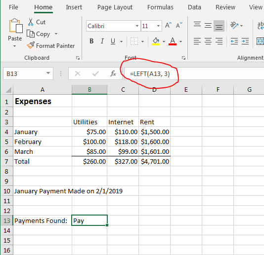
  (LEFT function example)

  The example uses the "Payments Found" cell to retrieve the first three characters, which are "Pay." If you specify a character count that exceeds the length of the string, Excel returns the entire string stored in the cell.

  The RIGHT function has the same syntax as the LEFT function including the same number of parameters, but the only difference is that the character count taken from the cell's string starts from the right side. Using the same cell in the "Expenses" spreadsheet, you can see the changes in the result when changing the LEFT function to RIGHT.

  Interested in learning more? Why not take an online Advanced Excel 2019 course?

  

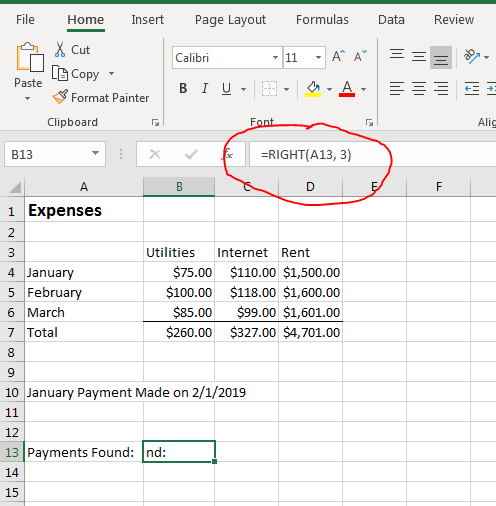
  (RIGHT function example)

  Nothing was changed other than the function used, because the LEFT and RIGHT functions have the same parameters. Since the character count starts at the right side of the string, the last three characters display in the selected cell. Just like LEFT, the default character number is "1," so if you only need the first character from the right side of a string, you can leave out this parameter.

  You will occasional want characters within a string that are neither on the right nor the left of a string. This is what the MID function can be used for. The MID function has one additional parameter than the LEFT and RIGHT functions, because Excel 2019 needs to know where to start and end the character retrieval where it's implied for LEFT and RIGHT functions.

  The MID function has the following syntax:

  MID (<text to search>, <location to start the retrieval>, <number of characters to retrieve>)

•          Text to search: The cell that contains the text to use.
•          Location to start the retrieval: The character number where you want to start the retrieval.
•          Number of characters to retrieve: The number of characters that you want to retrieve from the string.

  Just like LEFT and RIGHT, if you use MID to retrieve more characters than what's stored in the string, Excel will display the rest of the string from the starting point character.

  

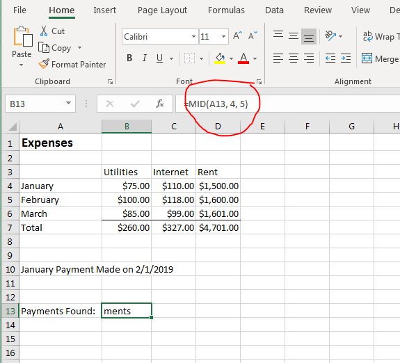
  (MID function example)

  Using the same A13 cell that was used in previous examples, the MID function in this example takes five characters from the string "Payments Found:" starting at the fourth character. The result is that "ments" displays in the selected cell. With the MID function, you can take as many characters from any location in a string, so it's more flexible than the LEFT and RIGHT functions.

  The UPPER, LOWER and PROPER Functions

  When working with string searches, you need to match a character's case. "Payments" and "PAYMENTS" are two different values to Excel, but you can change character case using the UPPER, LOWER and PROPER functions. The UPPER function changes all letters to uppercase. The LOWER function changes characters to lowercase. The PROPER function changes every word in a sentence or phrase to proper case, which means the first letter of every word is uppercase and all other letters in a word are lowercase.

  All three functions take only one parameter. The following is the syntax for the UPPER function:

  UPPER (<text>)

•          Text: The cell reference or text that you want to change to uppercase

  The text can be one character, a word, a short phrase or an entire sentence. If you reference a cell, the entire cell's content is changed to upper case.

  

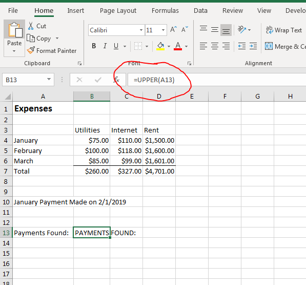
  (UPPER function example)

  Notice in this example that the text "Payments Found" is now all uppercase. If you have any special characters or numerical values in the string, Excel 2019 ignores them without issue.

  The LOWER function works similarly, but instead of capitalizing all letters, the string changes to all lowercase characters. The parameters are the same as well. The following is the LOWER function syntax:

  LOWER (<text>)

•          Text: The cell reference or text that you want to change to lowercase

  You can enter static text for the "text" parameter, or you can use a cell reference.

  

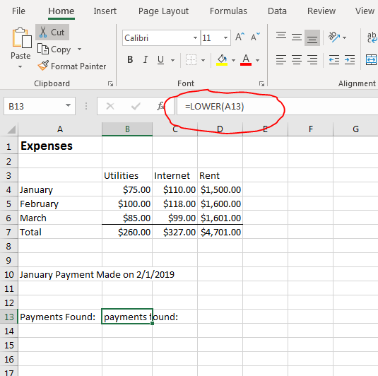
  (LOWER function example)

  Just like the UPPER function, the LOWER function changes all characters in a string to lowercase and ignores any special characters or numbers. If the entire cell is special characters or numbers, both functions ignores input, and nothing changes.

  The PROPER function works slightly different. Instead of changing all letters to upper or lowercase, the PROPER function changes the first character of each word to uppercase. This is commonly used when you have user-generated input exported to a spreadsheet. This data usually needs formatting, and you can change content to proper case for easier review.

  The PROPER function has the following syntax:

  PROPER (<text>)

•          Text: The text that you want to format 

  Notice again that PROPER has the same parameter syntax as the other functions, but the output is much different.

  

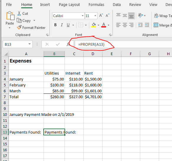
  (PROPER function example)

  Since the "Payments Found" string already has the first letters capitalized, no changes are made. If any one of these words were all lowercase, the first character would be capitalized.

  The SUBSTITUTE Function

  When you want to do a global find and replace in a string, you can use the SUBSTITUTE function to swap out one set of characters for another. It's a way to change data that's misspelled or when data requires certain characters added to a string.

  The SUBSTITUTE function has the following syntax:

  SUBSTITUTE (<text to search>, <text to find and replace>, <new text>, [OPTIONAL]<number of instances to replace>)

•          Text to search: The cell or text that contains the string to replace.
•          Text to find and replace: The old text that you want to replace.
•          New text: The text that will replace old text.
•          Number of instances to replace: If the text to replace is found more than once, you can specify the number of times to replace the string.

  The number of instances to replace is optional, so if you don't specify the number of times that the replacement should happen, Excel assumes that you want to replace all instances and will replace them all.

  

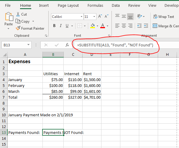
  (SUBSTITUTE function example)

  You can add any text as a replacement, and this example inserts the string "NOT" into the "Payments Found" string and changes it to "Payments NOT Found." The number of instances parameter was not defined in this example, because the term "Found" is only present once in the string. If there were numerous instances, all of them would be replaced since it was not specified.

  Using text functions in Excel will control user input and change formatting so that spreadsheets can be more easily read. It helps normalize data especially when it's user-generated. These functions will format and control text so that spreadsheets are more presentable before publication.