
A Brief Overview of Sparklines
Sparklines are simple charts, so they are only beneficial when you want to display a simple pattern in a row of data. If you need more advanced charts, you should add a graph in your spreadsheet, which is also an option in Excel. Sparklines give you a quick graphical representation so that trends in data can be quickly reviewed.
You have three different types of Sparkline graphs to choose from: line, column and win-loss. The type of graph that you use depends on the data display in a row. Line charts show trends in data where a win-loss chart just shows an up or down bar chart. A column chart also shows a trend in data by displaying a graphical representation of values stored in the selected cells. The type of chart that you choose will make it easier to visualize data, and you can always change the type of chart if you display.
Charts are also dynamic, so the visualization will change as you edit data in your rows. After you add a Sparkline chart, you no longer need to edit data or the selected cells unless you want to add more data to the chart. Once it's added, you can delete, change and add data to the chart's cells and Excel will automatically update the visual representation.
Adding a Sparkline
For this example, a line Sparkline will be used, but the steps to add a Sparkline chart are the same for the other two types. Line charts are the most common way to show data patterns. Using the "Expenses" spreadsheet, you can add a Sparkline chart to identify patterns for each payment type.
The first step to add a Sparkline chart is to select the cell where you want the chart to display. Usually, this cell is at the bottom of a column or to the far right of a row. With this example, the Sparkline chart will be at the bottom of each column to visualize payments for each bill. After you select the cell, click the "Insert" tab. You'll find a "Sparklines" section in the main menu where each type of chart is displayed as a button. Click the button for the Sparkline chart that you want to add, and the "Create Sparkline" window opens.
(Create Sparkline configuration window)
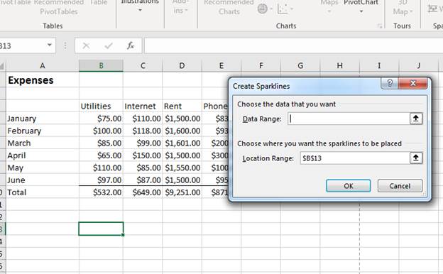
The first text box in the Sparkline creation window is the data range that you want to use for the chart. You can either type the cell range in the text box, or you can click the "up arrow" button and use your mouse to highlight all data cells. If you manually type a cell range, remember that the beginning and ending cell are separated by a colon character.
Since you've already selected the cell where you want the Sparkline chart to be placed, the "Location Range" text box is filled out already. If you decide to place the chart in a different cell, you can type this cell reference name in the "Location Range" text box. This text box also takes a range should you decide to play the chart in multiple cells for a larger visual layout.
After you make your selection, click "OK" to add the chart to your selected cell.
(Added Sparkline chart)
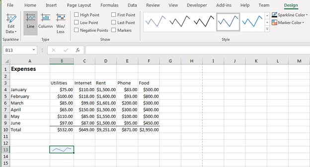
This adds one Sparkline chart to the first "Utilities" column, but you probably want to show a chart for each column to better understand the payments that you spend each year. You don't need to follow the steps to create a new Sparkline chart for each column. Instead, you can just copy and paste from the first cell with the Sparkline chart to all other rows. Excel will detect that it needs to change the range data for the chart to reflect the new column.
(All charts added and "Design" tab activated)
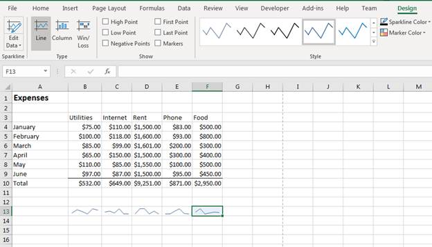
When you add a Sparkline chart, the "Design" tab is automatically activated, so you can stylize your spreadsheet graphic layouts. Using the tools in this tab, you can edit just about every aspect of your Sparkline charts from line colors, data, chart type and theme colors.
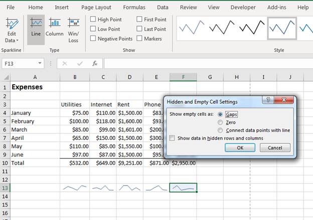
One issue that you might come across when working with large spreadsheets is that some cells within a column or row might not have any data. For instance, you might double-pay a month and get ahead with your Internet payment. You would then skip the following month and have no payment entered in a cell. If you include this blank cell in your Sparkline chart range, the chart will have a gap instead of displaying a continuous line. You can handle this by configuring Excel 2019 to connect the line regardless of a gap.
(Handling hidden and empty cells)
By default, Sparkline shows gaps for empty cells. You can also choose to plot the data as a zero value or "Connect data points with line." The third option will eliminate any gaps in your Sparkline line charts. Click "OK" to finalize and apply the changes.
Editing Colors, Styles and Themes
There are several notable sections in the main chart "Design" tab. In the "Type" section, you'll see three buttons that represent the type of Sparkline charts available. You don't have to recreate each chart if you decide to change the chart type. Instead, highlight the Sparkline chart that you want to edit, and then click the chart type that you want to use. For instance, clicking "Column" will change the selected chart type from line to column.
The "Show" section has several options to help certain data points stand out visually. Each option in this menu section has markers that will point out a low point, high point, and the first and last point. To add this design to your Sparkline charts, select the chart that you want to change and check the box to activate it.
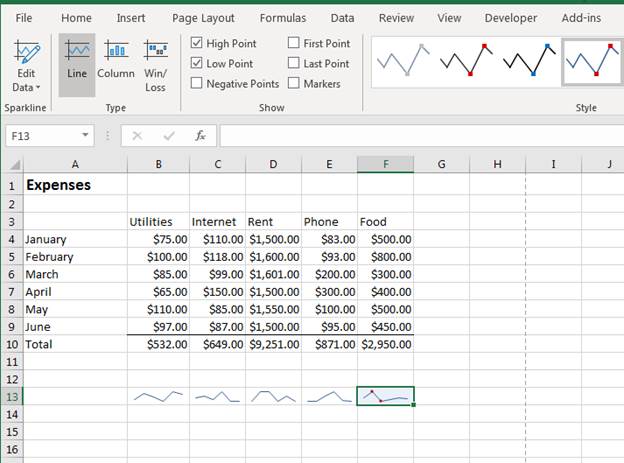
(High and Low point markers selected)
When you make these changes to one chart, you probably want to add them to other charts in your spreadsheet. You can repeat these steps to show markers or you can copy and paste the edited Sparkline chart from the one that you just changed to each additional cell. Excel 2019 will automatically make changes to reflect the right column range for each chart.
The "Style" section contains numerous themes with colors and border styles for your line chart. Since a line chart is what is selected, the themes shown in the "Style" section are all line styles. If you have another Sparkline chart type selected, the styles shown will reflect the chart type in the selected cell.
Scroll down the list of styles to find one that you like and select it. When you select a different style than what's show in the Sparkline chart, the changes immediately take effect and the new style is applied to the chart.
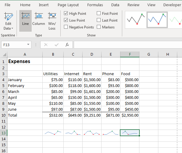
(New Sparkline style applied)
Styles are beneficial when you have multiple data points that stand out using markers. In the above example, low data points are marked in red and high points are marked in green. This change was done using Excel's premade Sparkline styles, but you can also customize colors and themes manually.
On the right side of the premade themes list is two buttons that let you manually style your Sparkline charts. The first one changes the line color and line thickness for the chart.
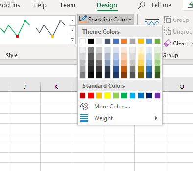
(Sparkline color options)
Click the button labeled "Sparkline Color" and a list of colors display in a dropdown. You can pick one of the standard colors and Excel changes the line color. If you don't like any of the listed colors in the dropdown, you can click the "More Colors" option to display a more advanced color picker. This color picker has finer color options, so you can specify the red, blue green mix for an accurate color that matches your own spreadsheet designs.
At the bottom of the dropdown has a "Weight" option. This opens to a submenu where you can see a list of line weight options. The default line weight is � points, so you can make this weight larger or smaller. You can also use a custom weight by clicking the "Custom Weight" option and typing a point value. Large weight values make the lines more visible, but they can also distort each data point if the cell where the Sparkline graph displays is small. If you have a win-loss or column Sparkline chart, the weight option will change to reflect the column attribute options.
Excel 2019 also has a marker color option. The default marker color is red, but you can change these dots that show on your lines to distinguishing colors to make them stand out. The color themes available in the premade list of styles have their own marker colors defined, but you can manually change them. The button to change marker colors is also on the right side of the style themes. The button is labeled "Marker Color."
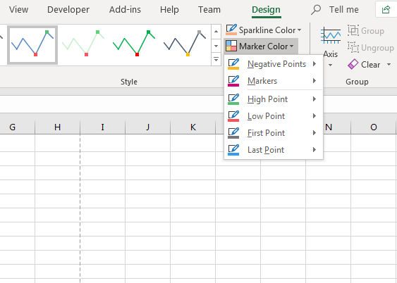
(Marker color options)
Click the "Marker Color" button and a dropdown of options displays. The options are set up in submenus for each marker type. Since the example only has high and low point markers, it makes sense to only change the colors for these two markers. Click the "High Point" menu option and a submenu of colors displays. The same color dropdown that displays for the Sparkline color options also displays for marker color options.
Click any one of the standard color options to change the marker color. If none of these standard colors will work for your spreadsheet design, you can click the "More Colors" option to open a configuration window. This window lets you pinpoint the exact color that you need for your design using your mouse or by typing in the red, blue, green values. Click "OK" when you've finally made your decision.
Edit Data
The final change that you can make to your Sparkline chart is its data. The "Edit Data" button in the "Sparkline" section of the "Design" tab displays the options to change chart data. Click the button and select "Edit Group Location & Data" to change the cell range used by the Sparkline chart.
Sparkline charts turn your regular spreadsheets into visually appealing output that can make evaluation of data much easier. They don't take up as much space as standard charts, and they are much easier to work with since Excel 2019 creates them on a basic range of cells and stored data.