
Data Validation
Excel has three types of data validation. In the "Data" menu tab, The data validation button can be found in the "Data Tools" section. The tools do not have textual labels, so you must hover your mouse over each button to find the data validation tool.
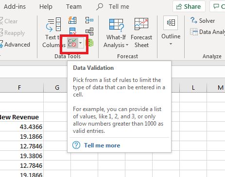
(Data validation button)
The data validation button has an arrow on the right of it that displays a dropdown with a list of options. The first one is the data validation option, so click this item from the dropdown list to open a configuration window. This window has three tabs where you configure the data validation when input is entered into a cell.
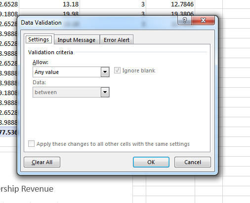
(Data validation configuration)
The "Settings" tab is the one that displays by default. By default, any value can be entered into a cell, but you can change this by clicking the dropdown and viewing the list of options. You can restrict input to whole numbers, time, text length, decimal, date or list. You can also customize the input that you will allow by selecting the "Custom" option.
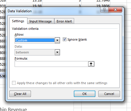
(Custom data validation)
Choosing the "Custom" option displays a formula text box where you enter your own formula. The formula will execute when a user enters data to validate that the value matches the formula's restrictions.
You might want to force users to enter at least some kind of value. For instance, if you have a quantity column, you might not want a blank cell. If the quantity is zero, then you might want users to enter 0 instead of nothing. By default, the "Ignore blank" checkbox is checked, but you can force a user to enter a value by removing the checkmark.
If you specify a numeric data validation rule, the "Data" dropdown activates, and you can then limit numeric values. For instance, you might want users to only enter values between 1 and 10. With this option, you can stop users from entering any value outside of that range. For this example, a restriction will be placed on the selected cell forcing the user to enter a whole number between 1 and 10.
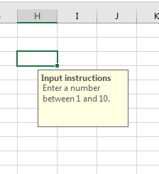
Click the "Input Message" tab to go to the next data validation step. This tab is where you configure the message shown to users before they enter a value. The message instructs the user so that they know what needs to be entered. Without it, a user would be frustrated as they try to figure out the value that must be stored.
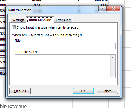
(Input Message configuration)
The default configuration has the "Show input message when cell is selected" checked. Without this option turned on, the user will not see the message when they select a cell. This option should always be turned on to make it easy for users to understand what must be entered.
The "Title" input text box is what shows at the top of the message box. The "Input message" text box is where you enter instructions for the user to read when the validation cell is selected. Should you want to start over, you can click the "Clear All" button at any time and Excel 2019 returns all configurations to the default.
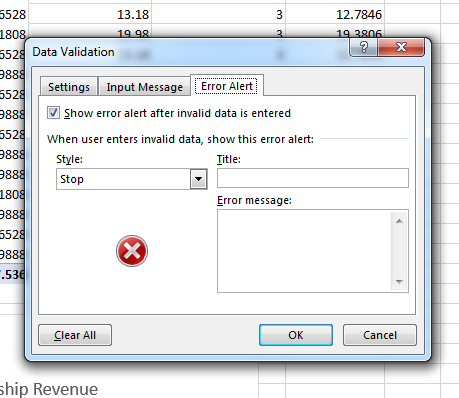
The next configuration tab is the "Error Alert" section. Click this tab to view the configuration options. This section is where you configure an error message should the user enter an invalid value
(Error Alert configuration)
In this configuration tab, you can determine the type of information that you want to display. The "Show error alert after invalid data is entered" checkbox should be checked, or your users will not see an error, which can lead to confusion and frustration. This option is checked by default.
The "Stop" style is the default, which gives users the intuitive red error icon. You can also give users a warning or just informational feedback. Choose the type of error that should be displayed in the "Style" dropdown. Just like the input message, enter a title and an error message in the "Title" and "Error message" text boxes.
After all three tabs are configured, click "OK" and the settings are saved. The validation rules you set are applied to the selected cell. The selected cell is what was chosen when you click the data validation button. Now, when you click the button, you see the input message that you set up in the configuration window.
(Input message)
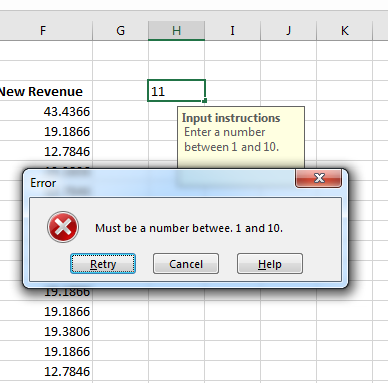
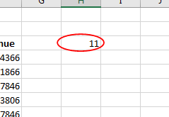
With the cell selected, you see the message in yellow. For this example, the user must enter a number between 1 and 10. To test the error message, enter the value 11 to see what happens.
(Data validation error)
After entering a wrong number and selecting another cell, Excel blocks the value and shows an error message. The error message you see is the one you configured in the data validation settings window. Click "Retry" to enter the right value or "Cancel" to close the window. The incorrect value is deleted, and you're prompted to re-enter the correct data.
Circle Invalid Data
In some scenarios, you might not want to add the jarring error popup window. The error message blocks a user from entering a wrong value, and the cell cannot be de-selected until the right value is entered. You can turn off the error message and allow a user to enter an incorrect value without getting stuck at the selected cell. This could be a way to allow incorrect values until the user is able to find the right value to enter. The option allows incorrect values, but still logs it as incorrect. Data validation tools give you a way to circle each incorrect value so that you can easily find them in your spreadsheet.
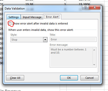
To disable the error message, select the cell with the validation rule added to it, and then click the data validation button. The configuration window opens with the current settings shown. Click the "Error Alert" tab.
(Disabled error alert)
To disable the error message, uncheck the checkbox labeled "Show error alert after invalid data is entered." Unchecking this checkbox is all it takes to disable data validation error messages. Click "OK" for the changes to take effect.
Select the cell with the validation rule added. Now, enter an incorrect value in the data validation field. Notice when you select another cell, the error message no longer displays. However, data validation is not turned off. Excel logs that this value is incorrect, but should you have dozens of these fields, it would be difficult to identify each on that has incorrect data.
The "Circle Invalid Data" option in the data validation dropdown menu helps you find any cell that doesn't contain the right data for the data validation rules configured. Click the dropdown and then select "Circle Invalid Data" to see results.
(Invalid data circled)
Excel searches through your spreadsheet and finds cells with invalid data, and then circles the ones found. In this example, the data validation rule requires a value between 1 and 10, so Excel circles the cell as invalid. This tool is beneficial when you don't want to restrict users from entering data but need to know when an invalid value is entered.
The circles will stay active until you change data, so Excel 2019 gives you a way to then turn off these circles. You would use this option when you just need a quick view of invalid data, but you're working on data entry and don't want to change entered data just yet. Excel's data validation tools have an option to remove all circles from the spreadsheet.
Click the data validation dropdown in the main menu and choose the "Clear Validation Circles" option. When this option is chosen, all circles are removed from the worksheet. You can always re-run the validation check on the spreadsheet again to see them again. These two options let you toggle the red circles on and off.
Remove Duplicates
With long lists of data, it's possible that you have unnecessary duplicates. Excel has a tool that lets you find duplicates and remove them so that you can get cleaner data than a bunch of cells that have unnecessary values. These values could cause your calculations to give you inaccurate numbers, so removing duplicates is sometimes necessary.
For this example, two columns of numbers were created and then selected. Click the "Remove Duplicates" button to open a configuration window.
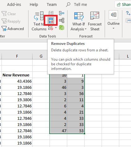
(Remove Duplicates button)
The configuration window lets you control the way Excel removes duplicates so that you get the right stored data without deleting information that could be important to your calculations.
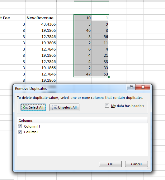
(Remove Duplicates configuration)
The columns listed are the ones you highlighted before you clicked the "Remove Duplicates" button. You can uncheck any column to remove it from the duplicates sweep. You can select as many columns or rows that you need to find duplicates. If your selected cells have a header, make sure you check the box labeled "My data has headers" to ensure that Excel does not include the header text in its duplicates process.
After you're finished with the configurations, click the "OK" button to run the procedure. When you run the procedure on two columns, Excel returns "No Duplicates Found." This is because the duplication checker bases its review on rows not columns. To fix this issue, copy all values from Column I to Column H. Then run the duplication checker on a single column. When the duplication check runs on a single column, Excel will now find the duplicate values, remove them from the column, and then give you a report.
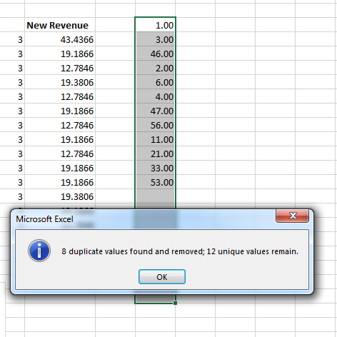
(Removed duplicate report)
If you decide that you need to find duplicate values across multiple columns, you can use conditional formatting features to highlight cells that contain the same value. When comparing values, you must also set the cell data type to the same across all cells. For example, if you compare a numerical value set as a decimal to a cell that contains a number but as a text data type, the duplication checker will not pick up on it being a duplicate value.
Text to Columns
Importing data from sources with unstructured data requires data validation and cleanup. One common import occurrence is full names importing into one cell. It's much easier to work with data when you have a separate column for first name and last name values. With combined first and last name values, it's much harder to run searches and query data based on last name. Excel 2019 has a feature named "Text to Columns" to automatically search through values delimited with a common character (such as a space character) and transfer values to two separate columns.
To get started with this tool, highlight the cells that contain space-delimited values and click the "Text to Columns" button in the "Data Tools" section.
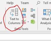
(Text to Columns button)
Clicking this button opens a configuration window where you define the delimiter and data source for the transition. There are three steps in separating values into their own columns, but you only need to finish the first two to separate name values.
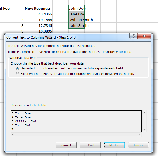
(Step 1 Text to Columns)
The first step is where you define if the values are fixed width or delimited. For most values, the data is separated by a delimited, so the "Delimited" option should be checked. Click the "Next" button to move to the next step.
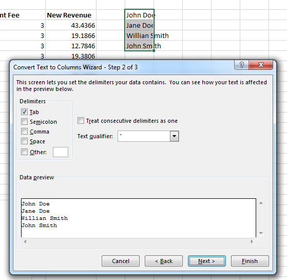
(Step 2 Text to Columns)
The default delimiter set is the tab character, but names have a space between the two values. Check "Space" and uncheck "Tab." Excel gives you a quick preview in the "Data preview" section at the bottom of the window.
At this point, you click "Finish" since you fully configured the tool but clicking "Next" will show you some additional options such as setting the destination data type.
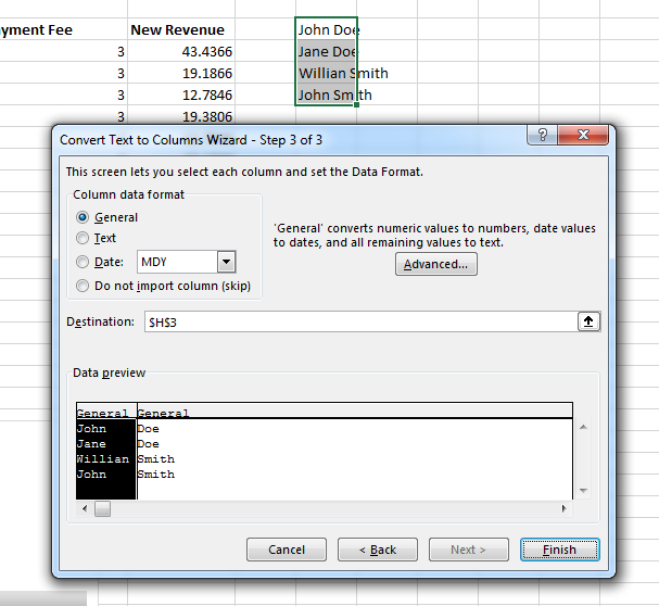
(Step 3 Text to Columns)
The "Destination" is set to the current column by default, but you can reset this cell value to another location on the spreadsheet. You can also set the data format, but with text values the "General" option is the right choice. Click "Finish" button to run the tool and separate the text values.
(Text to Columns results)
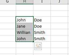
The result is that values are separated into separate columns. This example has two words separated by spaces, but if you have several words separated by spaces, these words will take one column per word.
Use these validation tools to clean up your data and change it in a way that makes it easier to query and structure. They can clean up thousands of records, and you'll need them when you import data from unstructured sources.