
Before you begin adding functions to a spreadsheet, you must know how to add them to a cell. When you type content into a cell, Excel translates it as textual information. To trigger Excel into translating content into a mathematical function, you must add an equal sign ("=") at the beginning of the cell's content. For each of the following functions, remember to add an equal sign before typing the function into a cell or Excel will see your content as textual.
The SUM Function
The SUM function is probably the most common mathematical function that you'll use in Excel Any basic totals and subtotals use the SUM function. This function simply adds all values within a range or specified in the function's parenthesis. The SUM function has the following syntax:
SUM (<comma-delimited cell addresses or ranges>)
(SUM function)
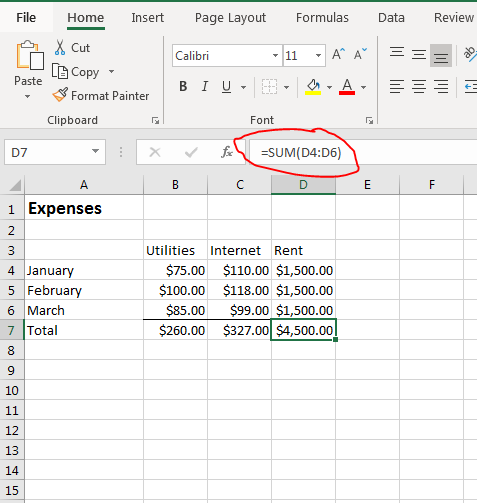
In the "Expenses" spreadsheet example, each type of expense is in a column and each month is a row. The total for each expense is shown at the bottom, and these cells use the SUM function. You could write the following in each total cell:
=D4+D5+D6
The above formula specifies to Excel that you want to add three cells and display the total. The formula only uses three cells in its calculation, but this can be very tedious if you have hundreds or thousands of cells to add up. The SUM function can take a range (or multiple comma-delimited ranges) of cells that you can specify using your mouse to highlight them.
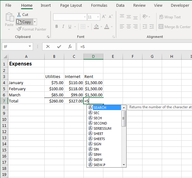
Excel has a type of Intellisense similar to Microsoft Visual Studio where it shows you suggestions and help when the software detects that you want to add a function. Type an equal sign into a cell, and a popup displays.
(Popup formula help)
When you are unsure of the function that you need, you can also click the "Fx" button to the left of the content text box or use the dropdown to the left of the content text box. The popup dropdown that shows happens after you type a letter after the equal sign. This dropdown is the quickest way to find the function that you're searching for. When you highlight a function, the text to the right of the dropdown gives you a brief description of the function. As you type more letters, the dropdown will narrow down your search.
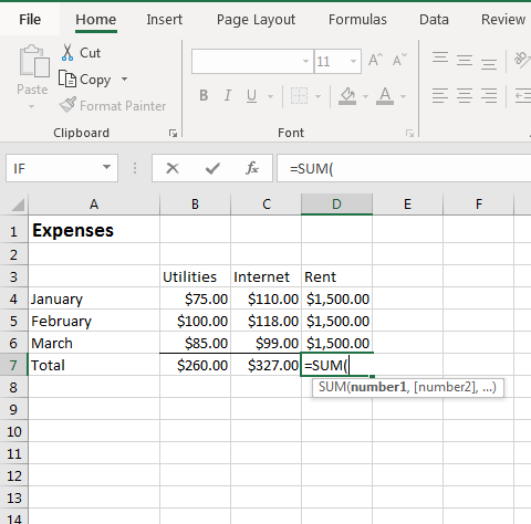
Once you find the function that you want (in this case, the SUM function), open the function with the first parenthesis and Excel then prompts you for input with a hint that displays the syntax that you need for the function to calculate properly.
(Excel syntax hint for SUM)
With large spreadsheets, you might not be able to see the range of cells that you want to add if you have several hundreds of rows. You could take note of the range before you add the function, but you could also use your mouse to select cells. With the SUM function opened, use your mouse to highlight all cells that you want to add. If the range is separated by cells that you don't want to use, hold the CTRL button and click each cell or cell range. After you're finished entering SUM parameters, add the closing parenthesis character and Excel displays the results.
If you want to type the SUM function's parameters, you enter the first cell in the range, a colon, and then the final cell in the range. When you use the mouse, Excel ensures that the proper syntax is used. The following formula would tell Excel to add up cells D4 through D6.
=SUM(D4:D6)
The SUMIF Function
Using other functions works similarly to the SUM function example. There are simple functions in Excel such as SUM, AVERAGE and COUNT. These functions perform simple calculations, but Excel also has more advanced functions that perform calculations based on multiple input. The SUMIF function is one of the more complex functions that will add a list of values based on a conditional statement.
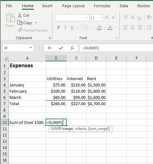
Using the "Expenses" example, you may want to add up values only if they reach a threshold. For instance, you would only add a rent payment to a cell if it's over the $1500 mark, which would indicate that you paid additional fees some months. You can do this by using the SUMIF function.
The SUMIF function takes the following parameters:
SUMIF (<range to evaluate>, <criteria>, <range to add up>)
If you forget this syntax, you can always click the "Fx" button to the left of the content text box, search for the function, and view a brief description and parameter list. When you type "=SUMIF(" into a cell, Excel begins the process of showing you what needs to be entered as function parameters.
(SUMIF hint)
The first parameter is the range to evaluate. You can either type the range into the first parameter and then type a comma, or use your mouse to select the range and then type a comma. If a function takes multiple parameters, you must always add a comma after each parameter except for the last one.
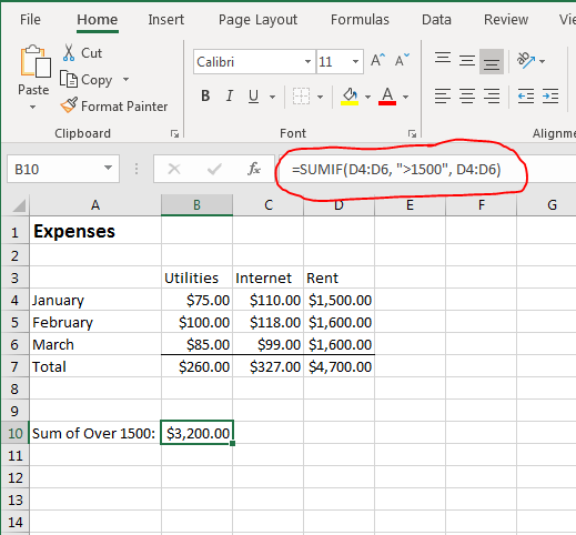
(SUMIF example)
In this SUMIF example, Excel evaluates cells D4 through D6 with the conditional criteria of ">1500" in each cell. Notice that the criterium is in quotes even though it's an inequality evaluation. Criteria can be greater than (">"), less than ("<"), and equals ("="). For very complex functions, you can use functions within functions for more advanced calculations.
The third parameter tells SUMIF which values to add up if the cell matches the criteria. Notice that the cell labeled "Sum of Over 1500" shows the results of two cells found to be greater than 1500.
The AVERAGE Function
All functions have a name with required parameters, but there are some Excel functions that you'll use more than others. The AVERAGE function is one of them that is used almost as consistently as the SUM function. This function takes the same parameters as the SUM function, but instead of adding values and displaying results, the AVERAGE function adds values, counts the number of cells used in the sum calculation, and then displays the result.
Using the "Expenses" spreadsheet example, you might want to know the average cost each month for your utilities. Utility costs go up or down depending on usage, so an average will help you identify your monthly budget.
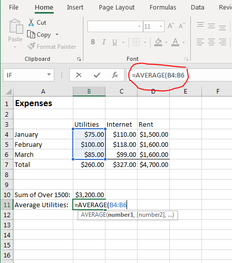
(AVERAGE function example)
In this example, the range B4 to B6 is added as the AVERAGE parameter. Instead of summing the values, the result shows an average.
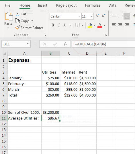
(AVERAGE function calculation results)
One advantage of using cell references in your formulas rather than actual number values is that any changes to these cell values will be updated dynamically in your formulas. Change a value in the utilities column and watch the value change in the "Average Utilities" cell.
The RAND and RANDBETWEEN Functions
Not every Excel function requires parameter input. The RAND function is a good example of a function with no parameters. This function gives you a random number between 0 and 1. The number is randomly generated by Excel and displays the result in the selected cell. In most cases, you'll use the RAND function within another function, but there are still occasions where you might want to simply display a random number as a factor in a calculation.
The RANDBETWEEN function lets you specify the two number ranges that you want to use to randomly generate a number.
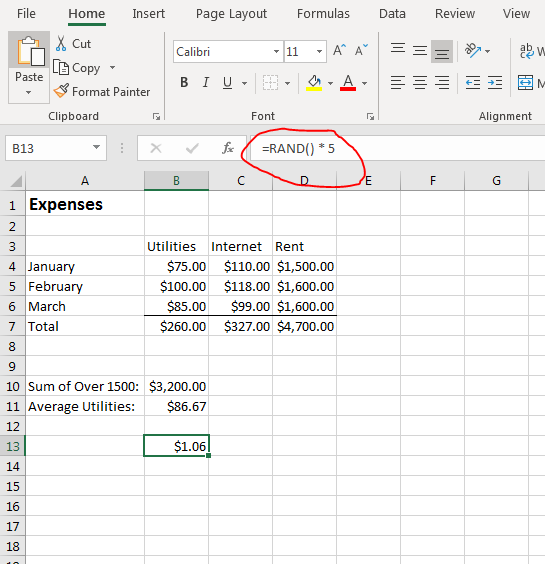
(RAND function example)
Using RAND, you can generate a random number and then use it in a calculation. Once the number is generated, it's set permanently. If you want to see the number generated, you should use just the RAND function in one cell and then reference that cell in your calculations.
If you want to specify the upper and lower limit for the range, you should use the RANDBETWEEN function. The RANDBETWEEN function has the following syntax:
RANDBETWEEN(<lower limit>, <upper limit>)
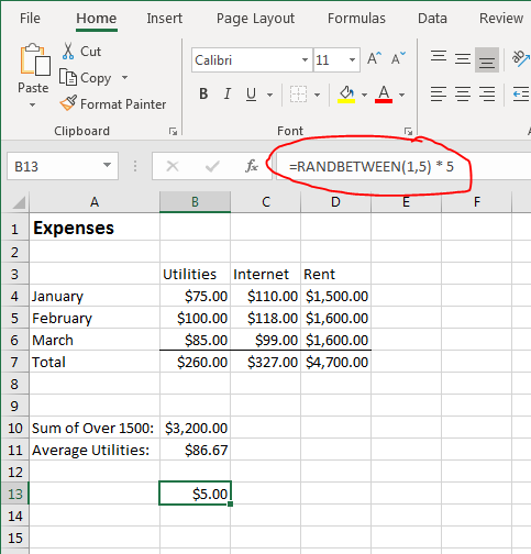
(RANDBETWEEN function example)
If you perform a quick calculation in your head from the example, you can see that the random number chosen by Excel is 4. Four is then multiplied by 5 and then the result is shown in the selected cell.
The COUNTIF Function
The SUMIF function adds values if the meet a specific criterion. You can do the same with the COUNTIF function except you count the number of cells that meet a specific condition. Excel 2019 has a simple COUNT function that counts the number of cells highlighted that contain numbers or functions that evaluate to numbers. The COUNTIF statement adds the conditional option to only count a value if it meets your criteria.
In the SUMIF example, only rent payments that exceeded $1500 were included. You may also want to know how many months of the year you paid more than $1500. This can be done using the COUNTIF function.
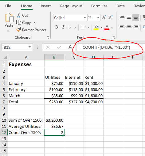
(COUNTIF function example)
If statements in any language are similar. You tell the application what you want to evaluate and the criteria for the condition. The SUMIF function has three parameters, but the COUNTIF only has two parameters since you just want to count the number of cells that meet a condition rather than summing values that meet a condition. As you can see from the example, only two rent payments were over $1500, so the cell labeled "Count Over 1500" displays a count of "2" values.
The ROUND Function
Excel 2019 has several rounding functions. The differences between them are the precision at which they round and whether they round up or down. The most commonly used rounding function is ROUND due to its parameter options. ROUND will round a number up or down and to the decimal point that you specify.
For many financial data, rounding to the nearest dollar helps with budgets and taxes. It's not uncommon to round to the highest dollar. Changing one of the rent values to a value with pennies added will illustrate the way the ROUND function works.
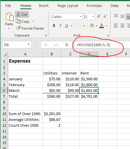
(ROUND function example)
The ROUND syntax is the following:
ROUND(cell, number of digits)
The number of digits parameter is how you control the decimal point at which the value is rounded and if the number is rounded up or down. In this example, the number of digits is set to zero so that the 50 cents added to the payment amount will round up to the next rounded integer. If you use a positive integer over 0 for this parameter, the function will round to the specified decimal point. For instance, a parameter of 1 will round to the tenth precision point. A parameter of 2 will round to the hundredth precision point.
Negative number of digits will round to the left of the decimal point. Zero will round to the first integer to the left of the decimal point. A -1 parameter will round to the second, and -2 will round to the third integer to the left of the decimal point.
The functions explained here are just a few available in Excel 2019. If you unsure if a function exists, remember that you can always click the "Fx" button next to the input textbox above the spreadsheet and search for the one that you need.