
Referencing External Worksheets
Referencing other data isn't limited to only the current worksheet. Excel 2019 gives you the ability to reference another sheet in the opened spreadsheet and even reference cells in an entirely different workbook. This gives you the ability to create a large network of workbooks that calculate and chart data without limiting results to only a single file.
If you recall, referencing cells requires a column name and a row number. For instance, the first cell in a spreadsheet is "A1" since the first letter in the alphabet is "A" and the first numerical row is "1." You still use these references along with new syntax when you reference external worksheets and workbooks.
Open an existing Excel file or create a new one. If you recall, a default worksheet named "Sheet1" is created when a new workbook is opened. Right-click "Sheet1" and select "Insert" from the context menu. Excel displays a new window with several objects available to add to a spreadsheet.
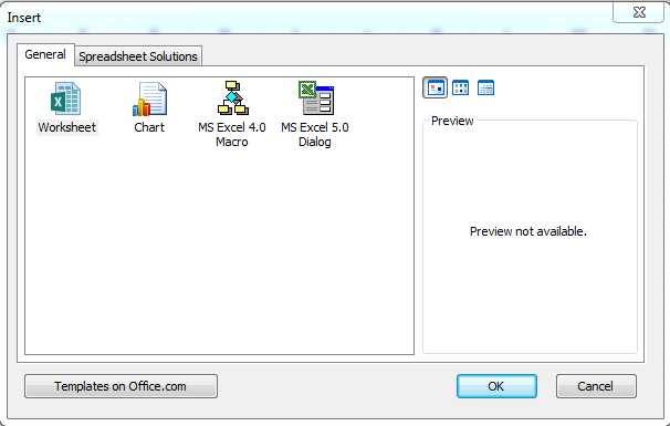
(Insert context menu)
Notice that the first option is a worksheet. Other options include a chart, a macro and a dialog menu. We'll cover some of these objects in future chapters, especially charting since it's a pivotal part of creating informational, aesthetically valuable reports.
Click the "Worksheet" option and a new spreadsheet with the name "Sheet2" is created. You can see this new worksheet tab at the bottom of your Excel workbook. For this example, the default worksheet names are used, but you can change these worksheet names by double-clicking the worksheet's name and entering a new name for it. You'll need to remember this new name or take note of it, because any new name will be used in formulas.
In Sheet1, enter "5" into A1 and "10" into B1. In this example, we'll multiply these two values and show results in A1 on Sheet2.
On Sheet2, enter the following formula into A1:
=Sheet1!A1*B1
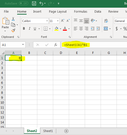
(Sheet2 referencing a cell in Sheet1)
Notice that the equal sign ( = ) is used to indicate that an equation is used rather than a literal string. However, notice that the result is zero. Because we're multiplying the two values "5" and "10," you know that the result is incorrect. When you reference another worksheet, every cell reference must have the sheet name in the equation. In the above worksheet, Excel multiples the value from Sheet1!A1 and B1 from Sheet2. Without the sheet name in the cell reference, Excel 2019 always assumes the value is stored in the current worksheet.
Change the formula in Sheet2's cell A1 to the following:
=Sheet1!A1*Sheet1!B1
The results are automatically updated, and the correct value is displayed.
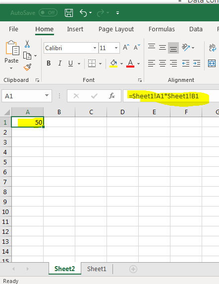
(Sheet2 referencing Sheet1 cells and displaying results)
The format for any external worksheet reference is the following:
=Sheet_name!cell_name
With any formula that uses an external worksheet reference, you must have this format. The exclamation mark tells Excel that the first referenced name is the sheet name and the second reference is a cell name.
Referencing External Workbooks
If you have a workbook fully created with several rows of data, you don't have to edit this workbook directly but rather create a new workbook that references this current data. Similar to referencing a separate worksheet in an opened workbook, you need to use a specific syntax in your formulas.
The following syntax is used for referencing an external workbook:
=[workbook_file_name]Sheet_name!cell_name
Notice that the workbook file name is in brackets. These brackets must enclose any workbook file name. The file name should also include the workbook extension such as xlsx or xls.
The first step to illustrate this concept is to create a new Excel 2019 workbook. Enter the value "2" into the A1 cell on Sheet1. Then, add the value "5" to B1 on Sheet1. Save the workbook to the same directory as your currently opened workbook. In this example, we're using a second file named "workbook2.xlsx" and stored it to the same directory as the currently opened workbook named "workbook1.xlsx" shown in previous examples.
Close the second workbook (workbook2.xlsx) and keep the first one opened. You can use the same workbook that we used in the previous examples. Enter the following formula into Sheet1 in cell A1:
= [workbook2.xlsx]Sheet1'!A1
Notice that brackets are used along with worksheet referencing syntax. In this example, no calculations are made. Instead, we just want to display the content of A1 in workbook2 to test that linking works.
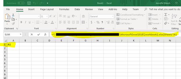
(Linking a cell to an external workbook file)
In the image above, the A1 text is shown, because Excel does not calculate results until you click another cell. After the current cell with the formula loses focus, Excel calculates the formula and displays results. Click any other cell other than A1 and notice that Excel pauses a second or two and displays "2" as the result. Because we entered "2" in workbook2.xlsx's A1 cell, your currently opened workbook also displays 2.
Notice that Excel also adds the directory tree to the external workbook file path. Since we stored the second linked workbook in the same directory as the currently opened one, then no directory path is needed. However, if you want to link a workbook in a different directory, then the path much be added. The brackets are only used for the workbook name.
= C:\mydirectory\[workbook2.xlsx]Sheet1'!A1 CORRECT
= [C:\mydirectory\workbook2.xlsx]Sheet1'!A1 INCORRECT
You can use calculations in linked workbooks as well, and the workbook name must be used in each referenced cell. Just like the external sheet examples, if you omit the workbook name in any part of your formula, Excel assumes the referenced cell name is the one from the current sheet.
Since we entered a second value in a cell named B2 in workbook2.xlsx, you can add this reference to the existing formula. In this example, we'll multiple the two values with a result of "10" displayed in the current cell.
The formula in the current spreadsheet is the following:
='C:\myfolder\MicrosoftExcel2019\[workbook2.xlsx]Sheet1'!A1*'C:\myfolder\MicrosoftExcel2019\[workbook2.xlsx]Sheet1'!B1
Because we entered "2" and "5" in these two cells, the result displays as "10."
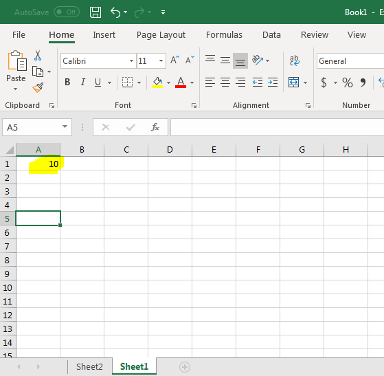
(Results from an external workbook reference and calculation)
One issue with linked workbooks is that any time the external file is changed, the values in the current workbook change. If you work in a team environment where multiple people have access to the file, it's important to realize that your workbook will also change. Additionally, if the linked workbook moves to another directory, the current workbook will display an error.
Leaving Comments for Revisions
In a team environment, it's not uncommon for a group of people to edit one Excel workbook. While reviewing files, you can leave comments for other users to make suggestions and changes to data. The "New Comment" function lets you create a "side" note in the spreadsheet for review. This functionality is found in the "Review" ribbon tab.
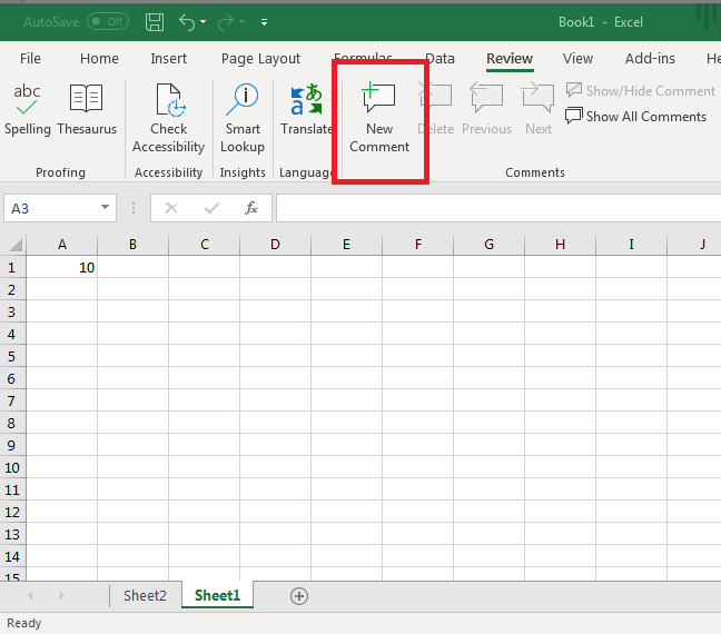
(New Comments can be made in the Review ribbon)
Click the cell that you want to comment on. In this example, only one cell has a value. Click "A1" and then click the "New Comment" button. A yellow note section opens where you can enter a note.
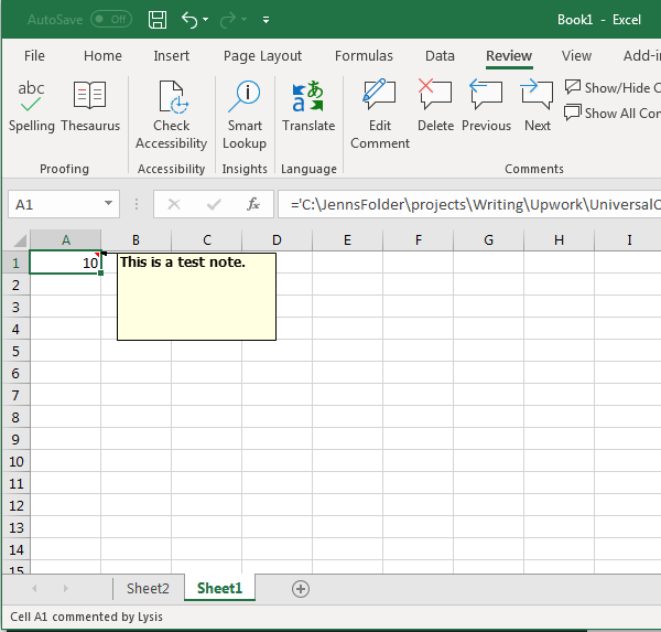
(Comment connected to cell A1)
With notes, a red triangle displays in the top-right corner of any cell that has a note attached. When these cells aren't selected, notes do not display. Click the cell with the red triangle indicator and notice that the note displays. This functionality is great when you don't want to edit and add text unrelated to data stored in the spreadsheet. Instead, you can store a note that does not interfere with other data asking a second person to edit values. It's also beneficial for spreadsheets where you need to set a reminder about the data you've entered.
Protecting Workbooks and Worksheets
Sharing workbooks is convenient when you trust each person to edit only cells that need to have changes, but it's not uncommon for users to share among untrusted recipients. For instance, you might use Excel 2019 to create invoices and send them to customers. You don't want customers to have the ability to change pricing and order information, so you can use the protection functionality in Excel to lock values. When this security feature is enabled, any third-party with access to your workbook must enter a password. You set this password when you lock selected cells. You can protect the entire workbook, a single sheet or a range of cells.
The protection functionality is found in the Review ribbon tab.
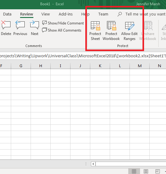
(Protect a worksheet or workbook)
To see what can be protected, click the "Protect Sheet" button. A new window opens where you can enter a password. Notice the list of options under the password text box.
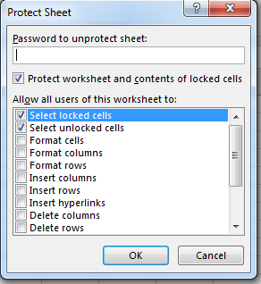
(Protect worksheet options)
These options determine what users are unable to do unless they know the password. For instance, you can stop users from inserting new columns into the worksheet.
You can protect the entire workbook by clicking the "Protect Workbook" button. A password is used to protect the entire workbook as well, and this option does not let you make granular permissions. If you want to disallow all changes, it's better to protect the workbook as a whole. If you want to protect only certain cells in a worksheet, it's best to password protect using the "Protect Sheet" option.
After you set a password, you can manually allow edits on cells using the "Allow Edit Ranges" function. Select a group of cells that you want to protect and click the "Allow Edit Ranges" button. This opens a new window here you can select cells again. Click "New" and select the cells that you want to protect.
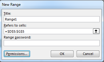
(Select a range to give permissions to other users)
This option gives you the ability to protect and release cells in a spreadsheet without blocking an entire worksheet with a password. Instead of giving permission to an entire sheet using a password, you can provide permissions based on the password given to a third party.
Editing workbooks and worksheets is common after you realize the benefits of storing data in Excel 2019. Referencing and protecting these workbooks also provides a way to determine the way others in your group can make changes. Use these basic features when working in groups that need to edit your spreadsheets.