The Goal Seek Tool

Excel's goal seek tool is the most common What-If analysis tool. When you have a table of data and want to make a change, you use the goal seek tool to make changes to your formulas to see results based on those calculations.

With the membership table, the net revenue of payments is displayed for each day in February. The calculation shows results for each revenue day so that the reviewer can see the actual revenue from each day that subtracts the payment fees. What if the payment fees changed? You might have a payment processor that you're reviewing that has higher fees or possibly one that has lower fees. How does this change your revenue? You can answer these two scenario questions using a goal seek What-If analysis.

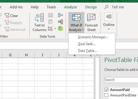
Excel 2019 has three What-If analysis tools. Goal seek is just one of them. The tools to use Excel's What-If features can be found in Excel's "Data" menu. Click this menu tab, and then you'll find the "What-If Analysis" button in the "Forecast" section.

(Whiat-If Analysis button)

Click the "What-If Analysis" button and a dropdown of options displays. These options are the three different tools that you can use for your What-If analysis. For this example, click the "Goal Seek" option.

(Goal seek configurations)

Before you perform a goal seek, you have a few requirements that you must follow before the tool will work. The example uses a pivot table to display data, but goal seek cannot change pivot table data. For this reason, a "Payment Fee" and "New Revenue" columns were created. The payment fee represents the percentage for payments. The new revenue column represents the total amount of revenue by subtracting the payment fee percentage from the gross payment amount.

When working with goal seek tools, the target cell must be a formula. This is because the goal seek tool will take your target value and temporarily change the values in your formula to reach your target scenario.

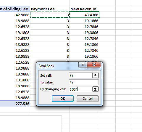
In this example, the scenario identifies the payment fee that you need to use to get to a specific amount. The net revenue currently for the first cell in the "New Revenue" column is 43.4366. This is the cell that contains the formula that calculates how much net revenue is made by subtracting the fee percent from gross revenue. The "Set cell" input text box must contain a cell with a formula, and the E4 column has the formula requirement.

The "To value" input text box is your target amount. You can run several goal seek evaluations on your worksheet data, but you would need to change values and use multiple goal seek scenarios. For this example, the goal 42 is set to see the maximum threshold for a payment fee to keep net revenue at 42 from the original charge amount.

The cell that contains the payment fee that can be altered is D4. The "By changing cell" input text box is the value that you want to alter. For this example, the payment fee is what will change to determine the fee that would result in net revenue of $42.

After you enter your goal seek values, click "OK," and Excel 2019 changes the values to display results.

(Goal seek results)

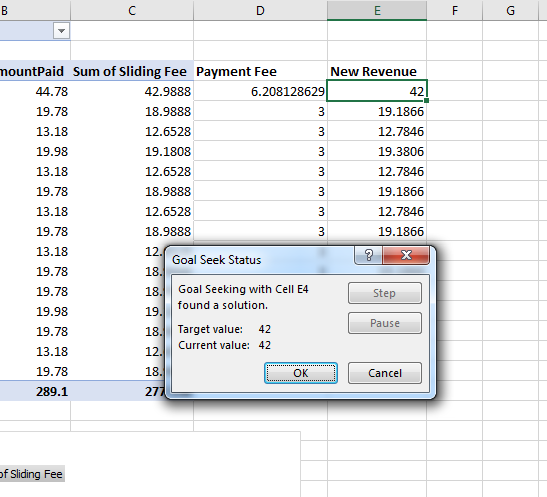
Goal seek searches for a value that would match your scenario results. In this example, the status window displays a notification that it was able to find a value fit suited your requirements. In the spreadsheet, Excel changes the results so that you can see the values that need to change to reach your goals.

In this example, payment fees were increased to examine a threshold for a payment fee that would keep the total net revenue at $42. The result was that payment fees could increase to up to a little over 6% and your total net revenue would not go below $42.

The "Goal Seek Status" window has a "Step" and "Pause" button. With some complex goal seek scenarios, the What-If tool won't be able to find a value that will match your proposed end result. You can use the "Step" button to add another step to the goal seek or use the "Stop" button to cancel the goal seek procedure and change the values for each input option.

The Scenario Tool

The goal seek tool lets you review one scenario and enter values for one end result. The scenario tool takes this a step further and lets you have multiple values and goals to find variations of your projections. To open a scenario configuration window, click the "Data" tab and then click the "What-If Analysis" button in the "Forecast" section. Clicking the "Scenario Manager" option in the dropdown menu will open a configuration window where you set up your scenarios.

(Scenario Manager window)

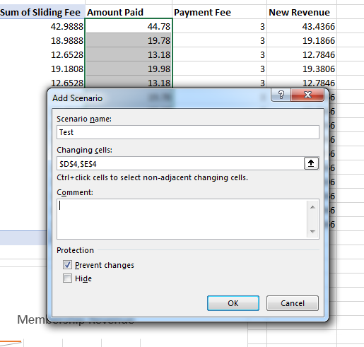
Because scenarios let you put together several projections, you have a much more complex configuration window when you work with scenarios. Click "Add" to create your first scenario based on the data in your spreadsheet. This example uses the data from membership charges, payment fees, and net revenue by subtracting fees from gross revenue.

(Add scenario)

Because a scenario lets you review several projects with multiple values, you can enter multiple cells in the "Changing cells" input text box. You can also add cells into this text box by using your mouse and clicking each cell in the worksheet.

Excel 2019 automatically fills in your name with the date the scenario was created in the "Comment" input text box. You can leave this text box blank or add your own comment to organize scenarios when you have several that you want to review. Give your scenario a name by entering a value in the "Scenario name" input text box. When you review a list of scenarios in the future, this name will help you find the one that you're looking for.

When you are finished configuring your scenario, click "OK" to create it. Now, it's time to enter the values for the selected cells.

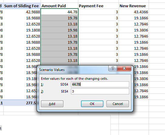
(Scenario values)

The advantage of a scenario over a goal seek is that you can change values in multiple cells, and the next window after creating a scenario is where you configure the values for each cell that you chose to change in the previous window. The default values are the ones that are already entered.

Each cell that you configured in the previous window is displayed with an adjacent input text box where you enter your new values. You can add multiple values, enter just one and leave the others, or any other combination of new values that match your scenario. In this example, the payment fee of 3% is changed to 2% with a total revenue value of $45. Click the "OK" button when you are finished entering new values.

After creating a scenario, you're returned to a window where you can see a list of all your configured scenarios.

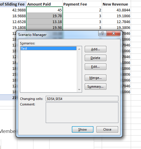
(List of scenarios)

From this window, you can edit, delete or add another scenario. This window is also where you can activate the scenario and view the results of your calculations. Click the scenario that you want to view (in this case "Test) and then click the "Show" button at the bottom of the window.

Clicking "Show" in this example changes the payment fee in the first row to 2 and the total amount paid as 45. The end result is the new revenue value. This value changes to a slightly higher amount. If you want to create another scenario with different values or additional cells to change, you can add another scenario with various changes. With scenarios, you aren't bound to only one goal with one variable input parameter. You can store multiple scenarios to quickly see the various ways that you can make revenue or manipulate costs so that you make your goals.

When you are finished with your scenario values, click "Close" to exit the window.

Data Tables

With scenarios and the goal seek tools, you set up cells with data that changes based on the variables that you set. For instance, using the payments and fee expenses, you might want to allocate a section of your worksheet that displays a list of possible revenue data points and the net revenue results for a specific payment fee. This example uses a 3% payment fee and then displays several data points with resulting net revenue values.

To create a data table, you first need to set up your column of data.

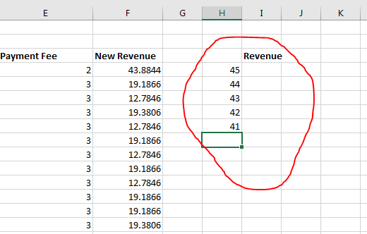
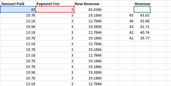
(Data table test data)

In this example, a column of revenue values is set up from $41-$45. To the right of each value is a blank cell with the column header "Revenue." This column is where the results of your data table calculations will display.

To create the data table, click the "What-If Analysis" button in the "Forecasting" section of the "Data" menu tab. Select "Data Table" from the dropdown menu and a configuration window opens where you can set up your data.

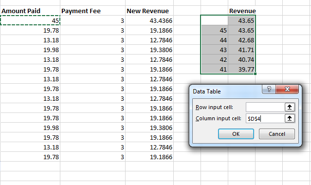
(Data table configuration)

Before you set up the table, you must enter the formula in the first cell under the column label. In this example, the first cell under "Revenue" with the value of 43.65 contains the formula =D4-(D4*E4/100) to calculate the first value in the data table. This formula tells the data table how to calculate the other values.

You must also select the two columns that contain the variable values and the cells to the right of them where the results will display. Make sure you include the cell that has the formula, or the data table will be unable to calculate a result regardless of the number of values you enter.

Data tables have two input text boxes that configure them with your selected data. The "Row input cell" text box is where you specify the cell that contains static information for each formula. Since this example will show different net revenue values for a static 3% payment fee, the "Row input cell" text box should be the cell with the payment fee, which is cell E4. However, this data table will use the column row text box.

The "Column input cell" text box contains the original first value 45. The "Row input cell" input text box can be left blank since it won't be used. Click "OK" and Excel uses the stored formula to configure the values in each row and displays the result in the right adjacent cell. For each column input, the calculation is made and then the results show in the table.

(Data table results)

When you apply the configurations to your data table, the window closes, and you can see the formulated values in the column you chose. With data tables, you can identify values that are used in the calculation because Excel 2019 highlights them in red and blue. This lets you quickly identify which values are used in calculations so that you can understand the information displayed in your worksheet.

Data tables are somewhat different than goal seek and scenario tools, because you can only use static values that are then used to calculate results from a list of input values that you specify in a table. Any alternative formats will fail, and Excel 2019 will give you an error and will not let you complete the data table configuration.

Excel will not let you simply redefine data table data. Once you create it, you must keep it on your worksheet unless you decide to delete it. You can clear a data table by highlighting all column data and pressing the "Delete" key. After you delete the table, you can then redesign and add new configurations to a new table that displays your information.

What-If tools in Excel help you determine the right direction for your finances and business. These tools are beneficial when you have data and want to make a change but you're unsure of how those changes could result in your financial projections. Excel's What-If tools are powerful features that can be useful when you want to know what could happen when data changes in your information.