When Would You Use Solver in Excel?
With the Goal Seek tool, you found values that can be used to determine an outcome. The outcome was a set value that Excel then used to calculate another value that would help you define your solution. It's a simple What-If analysis tool that can be used for basic projections, but you might have a more complex scenario where you are unsure of multiple variables including your goal. This is where the Solver tool comes in handy.
Solver helps you find a projection or solution to your problem using a group of cells and a formula cell (called an objective cell). These cells contain a formula for your main calculation and values set as maximum and minimum called constraints. Decision variable cells, constraints, and your formula work together to find a solution to your problem with a result that you're searching for. Use the Solver tool when you have variables that you're unable to pinpoint accurately and need more loosely defined constraints.
Adding Solver to Excel
Since Solver is a Microsoft add-in tool, you can download and add it directly from the Excel 2019 interface. Click the "File" tab, and at the bottom of this window, you will find the "Options" button.
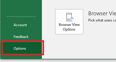
(Options button)
After you click this button, a configuration window opens. Click the "Add-ins" button in the left panel to see several add-in configuration options.
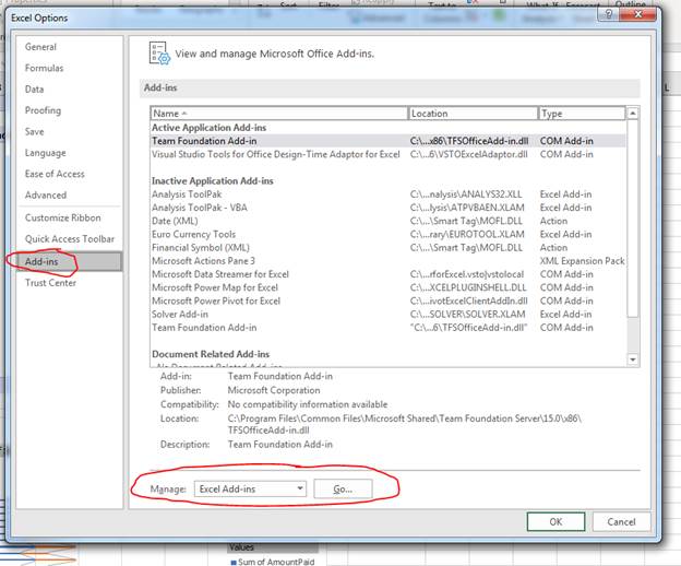
(Add-in configurations)
In this window, you can see a list of add-ins installed in Excel. Add-ins are available to all Microsoft Office applications provided they can be used with the application's workflow. In this list, look to find "Solver Add-in." If you find it, then it's already installed. If you do not see it in the list, click "Go" next to the "Manage" dropdown with "Excel Add-ins" selected. Another configuration window opens.
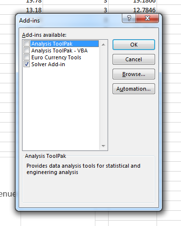
(Add-ins installation)
Check the box next to the add-ins that you want to install. For this example, check "Solver Add-In" and click "OK." After you click "OK," Excel 2019 installs the Solver add-in and it can now be used with the Goal Seek tool. Excel adds the Solver tool button in the "Analyze" section of the "Data" menu tab.
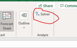
(Solver button)
Working with the Solver Tool
With the membership fee test data, you might have a specific revenue that you want to make after fees. You can go lower or higher with the fees that you have, but you aren't sure what type of revenue you can make based on the current numbers. The Solver tool can make this decision for you where you can set upper and lower limits with a set goal that the tool solves.
Before you begin, you need an objective cell. The objective cell is the number that you want to get to, and it must be a formula. The formula calculates your basic, current data from the spreadsheet.
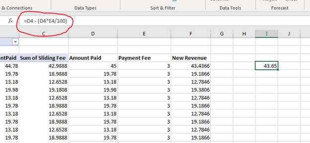
(Formula cell)
With the formula cell created, you can now click the "Solver" button and get started. Click the "Solver" button in the main menu to open the configuration window.
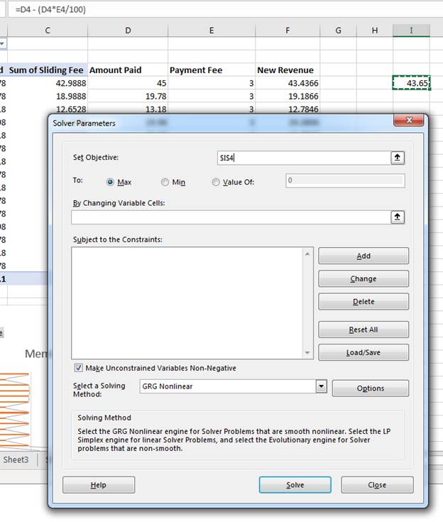
(Solver configuration)
The configuration window has several parameters where you set up your scenario values. The first input box is the "Set Objective" value. In this example, the formula cell is located in the I4 cell, so it's entered in the input text box. Any data must be in the same worksheet to be valid parameters for the Solver tool.
The next set of parameters is the "To" section. This section lets you determine if you want to create a scenario with a maximum value, a minimum value or an exact value ("Value Of"). For this example, a minimum revenue number will be used because the question is how much of a fee can be applied before sales numbers are too low to meet required net revenue.
The "By Changing Variable Cells" section is where you set your decision cells. You can have up to 200 decision cells with the Solver tool. This section is what makes the Solver tool more flexible and powerful than a simple Goal Seek calculation. With these values, Excel will determine what values can be used to reach the goal set in the "Set Objective" section. For this example, ten decision values will be used. The values will be between 1 and 10.
The "Subject to the Constraints" section is where you set the constraints for the Solver solution. For instance, with membership revenue you might not want it to drop below a certain point. You can set this constraint in reference to the formula cell to find solutions that don't go below a specific amount. This example will use the $15 minimum amount.
To add a constraint, click the "Add" button in the "Subject to the Constraints" section.
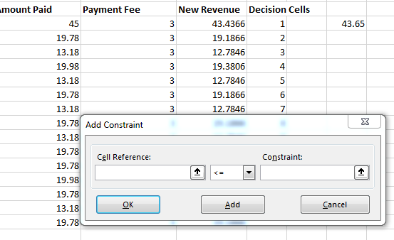
(Add constraint)
The window that opens is the constraint configuration window. This window lets you choose a cell, an inequality or equality statement, and then the value that you want to constrain. The inequality dropdown has several options where you can match types, values and comparisons. After you enter the required values, click "Add" if you want to enter another value. The constraint is added, and you can enter a new one. If you are done with the list of constraints, click the "OK" button to close the configuration window and return to the main Solver configuration window.
Before you finish configuring the Solver tool, you must decide on the solving method. This dropdown is located in the "Select a Solving Method" section under the constraints section. The type of solver method that you choose will determine the outcome.
The solving method is its own complex formula, so the choice you make will determine speed of the solution as well. While speed is not an issue for small problems such as the current example, if you have 200 decision cells with numerous constraints, time becomes a factor. Each algorithm has its own complex formulas, so you could wait several minutes before you find a solution for some scenarios. Here is a basic explanation for each algorithm.
GRG Nonlinear: The "GRG" in this algorithm's name stans for "Generalized Reduced Gradient." It's the fastest of all three algorithms, so if you have complex constraints and requirements, this algorithm might be the best solution. It's also the least optimal as the GRG Nonlinear algorithm, so it comes with a downside. GRG Nonlinear will not find global optimal solutions when initial factors are not optimal. Any IF, VLOOKUP or absolute functions could also cause problems for this method.
Evolutionary: Excel's Evolutionary algorithm is much more accurate and robust than the GRG Nonlinear algorithm. The Evolutionary algorithm creates a set of random numbers. These population numbers and then narrowed down into another set of population numbers. Each narrowed-down population number set is called an offspring, and each offspring is reduced until Excel is able to find the best solution. This solution is much more accurate, but again the disadvantage of this algorithm is that it takes much longer than the others. If you have plenty of time to wait for a solution, this is the algorithm that you should use with the Solver tool.
Simplex LP: The Simplex LP algorithm is very limited, but it's beneficial if you are only looking for linear solutions. It's a fast method due to its limitations, but its advantage is also that it finds a global solution that is likely on target to the result that you're searching for. When you have very simple solutions that rely on linear values, you should use this one as it's the most accurate of all other algorithms.
With these basic explanations, you can choose a method for your calculation. If you're just reviewing the way the Solver works, you can leave it as the default GRG Nonlinear choice since this one will find a solution, and it's the fastest without the linear limitation that Simplex LP has with its requirements.
When you are finished making your constraints and setting Solver configuration, click the "Solve" button and wait for the tool to find a solution. Because this is a small example, it will not take long for Solver to find a solution if there is one. When the Solver tool is finished, another window displays showing more options and letting you know if a solution was found.
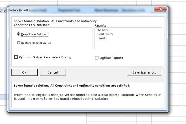
(Solver solutions window)
The results window tells you at the top if a solution was found. If one was not found, you can check the box labeled "Return to Solver Parameters Dialog" to go back to the configuration window and enter different values. The Solver might not be able to find a solution due to the parameters you entered, or the solution that you want is impossible. This is the advantage of the Solver - it can help you determine if a result is feasible, and if it is feasible, how you can achieve it using algorithms and numbers.
If the Solver finds a solution, it creates a report that you can view on your screen. The default selection is to "Keep Solver Solution" so that you can see the results. You can also restore original values by choosing the "Restore Original Values" if you are unhappy with the Solver results.
The "Reports" section shows you what the Solver has for you when it prints out reports. Choose one of the reports that you want to see. For this example, the "Answer" report is selected. When you are finished choosing your options, click the "OK" button to see the results. With a report is selected, a new worksheet is created where you can see the results of your Solver solution. The worksheet has the worksheet name "Answer Report 1." Click the tab to view your report.
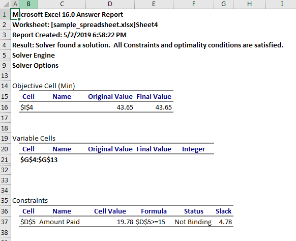
(Answer report)
With the Answer report, you can see the "Slack" that gives you the answer of how much payment fees you can pay before you reach the threshold set in the Solver configuration window. This report is beneficial when you have several scenarios and need to review each one in separate reports. The Answer report shows you the parameters, constraints and objective cell values that you can review compared to the solution that the Solver came up with.
If you want to see another report, click the "Solver" button again to open the configuration window. Click "Solve" and the results window will display. This time, click the "Sensitivity" option in the "Reports" section and then click "OK." Excel will close the window and generate a report that displays in the next tab. The tab is automatically given the name "Sensitivity Report 1." Click the tab to see this report.
(Sensitivity report)
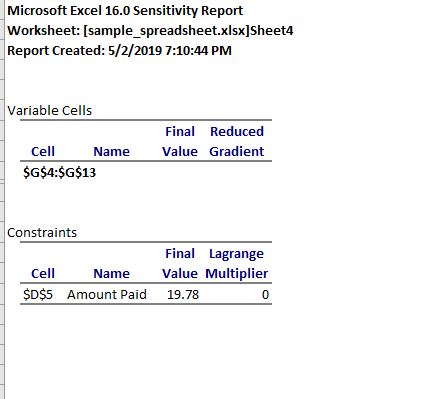
Because this example is so small, not much can be seen from the sensitivity report. This report shows you how much your results change with slight differences in variable numbers You can use this report when you have numerous constraints and want to see what will happen with just a minor tweak in your data.
Next, take a look at the Limits report. Click the "Solver" again (make sure you switch back to the worksheet that has your data or the configuration window will be empty). Click "Solve" again and the results window displays. Again, a worksheet is created with the name "Limits Report 1," and you can click on the tab to view the report.
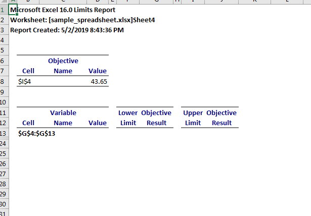
(Limits report)
When you work with maximum and minimum values, the limits report allows you to see the changes in the objective function when other factors remain constant. Because the solution for the example is basic with only a few decision cells, this limit report does not show any variable changes but if you had numerous constraints and decision cells, you would see objective options that would match your objective.
The Solver tool is an advanced way for you to find solutions to your questions. You can use the simple Excel Goal Seek tool, but when you need complex solutions with numerous constraints and factors that can produce a result, you use the Solver tool. Excel 2019 has this tool as an add-in free for you to use.