The Formula Tab

Excel does an excellent job of organization features and grouping them into menu sections that make sense to a new user. The "Data" tab contains all features to create and manipulate information stored in a table either in a local spreadsheet or in a remote database. The "Formula" tab contains all the features to work with formulas including the ability to audit and troubleshoot them. Before you publish a spreadsheet that contains several formulas, you should use these features to review them for any errors.

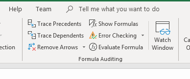
Click the "Formula" tab to view what it offers.

(Formula Auditing menu section)

The left side of the "Formula" tab contains buttons labeled with formula categories. Click one of these categories, and you can choose one of the formulas to fill a cell. In the center section of the menu, the "Formula Auditing" group contains the features to troubleshoot and audit formulas throughout the file. Each one of these tools can help you find what could be critical errors in your calculations.

Trace Precedents

If your cell is retrieving data from the wrong location, then your calculations would have errors. The "Trace Precedents" feature shows you the cells being used by a selected formula.

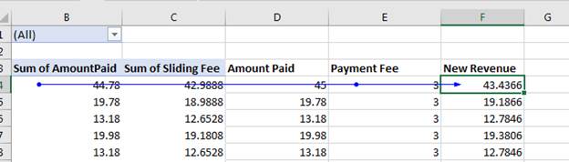
With the membership fee data, a revenue column calculates the net revenue by subtracting the payment fee from the gross payment. By using the trace precedent tool, you can see the cells used in the net revenue formula.

Click the cell that contains the formula, and then click the "Trace Precedents" button.

(Trace Precedents)

The trace precedents tool draws a line from the starting referenced cell to the formula cell. In this example, the first cell used in the formula is B3. There is a dot on the line that indicates the cell is a part of the formula. The line moves across the row to the "Payment Fee" column where another dot indicates it's a part of the formula. Notice that there is no dot on the "Sum of Sliding Fee" and "Amount Paid" columns even though the line runs across them. This indicates that the two columns are not a part of the formula.

You can only choose one formula cell at a time with the trace precedents tool, so it can take time to review all formulas, but it's beneficial if the cell contains a long, complex formula. Having a visual representation of the cells involved can better help you identify errors.

Trace Dependents

Changing just one value can make considerable changes to your data when multiple cells reference it directly and indirectly. The "Trace Dependents" tool identifies what formula columns reference a data cell.

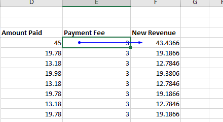
In the example, the "Payment Fee" column is referenced by the "New Revenue" formula cell but suppose that you don't remember what columns reference the value. Click the cell that contains a payment fee value and then click the "Trace Dependents" button.

(Trace Dependents)

Now the line drawn is from the payment fee cell to the formula cell that contains net revenue. The dot indicates that the cell selected is used in the formula.

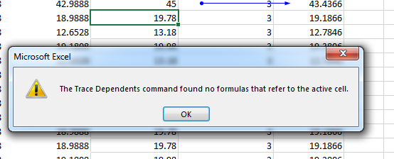
Not every cell will be a part of a formula. Click a value in the "Amount Paid" column, and then click the "Trace Dependent" button again.

(No trace dependents)

When no formulas reference a selected cell, the trace dependent tool lets you know with a popup. Click "OK" to close it the window and return to your spreadsheet.

Remove Arrows

The arrows for the trace functions stay visible on a spreadsheet until you remove them. You can click each cell and run a trace until you have arrows that indicate all dependencies and precedents. However, once you're done you need a way to remove the line arrows. You can remove them by simply clicking the "Remove Arrows" button in the "Function Auditing" menu section.

Show Formulas

In large worksheets, it can be difficult to identify formula cells when they just contain values that display from the calculation. You can separate standard value cells from formula cells by clicking the "Show Formulas" button. Clicking this button will expand cells so that they display the formula so that you can review the information.

Combine this feature with the trace functions, and you can see the values used in a formula and then the formula that calculates results.

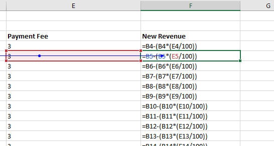
(Show Formulas)

One issue with this tool is that long formulas will expand a column to where it's difficult to view the rest of the data. You'll need to resize columns if they take up too much space in the interface. However, this tool let's you find formula columns much more quickly than clicking each cell one-by-one.

Error Checking

Auditing tools identify formulas, trace dependents and precedents, but they don't help identify errors. Luckily Excel 2019 has error checking as part of its auditing features. There are two features in the error checking toolset. Click the arrow next to the "Error Checking" button to see both features.

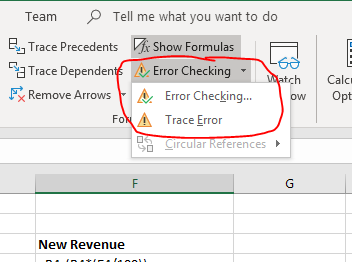
(Error Checking)

With small spreadsheets, it's easy to take a quick look at your formula fields and identify the ones returning an error. If you have large spreadsheets with numerous columns and records, it could be hard to find the one formula that references a null value and displays an error in its calculation. Error checking tools are used to find them instead.

Click the "Error Checking" option and a configuration window opens.

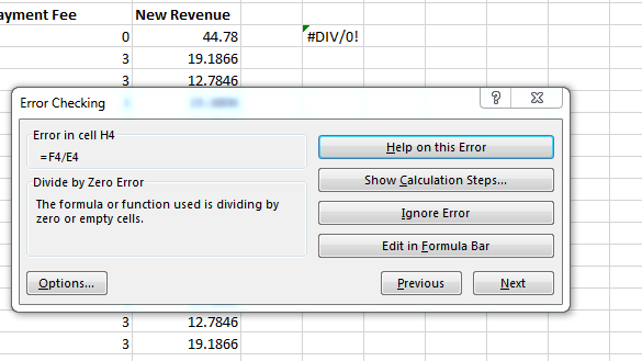
(Error Checking)

Error checking might find several issues, so you can click the "Previous" and "Next" buttons to scroll through each one. Each error has a section on the left that displays the formula, explains the issues, and tells you the cell where the error is located.

The section on the right has options to help you decide what to do. The issue with this example is that the cell contains a formula that divides a value by zero. If you're unsure how to fix this error, click the "Help on this Error" button to get some advice. This button triggers your browser to open a Microsoft web page that will give you more information about the error.

The most helpful tool in the error checking toolset is the button labeled "Show Calculation Steps." This button shows you the formula with its reference cell values. By seeing the values used in the formula, it can help you identify the error.

(Show Calculation Steps)

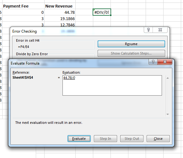
In the left section of the window, it shows the cells referenced in the formula. Then in the "Evaluation" section, you can see the actual values and not just the cell references. Excel can help you even further by stepping through each cell reference. Click the "Evaluate" button to start the evaluation tool.

The first step in the evaluation shows the error that you see in the cell already, so click "Restart" to give yourself the ability to step in and out of the calculation steps. The first step is to take a look at the cells referenced in the formula.

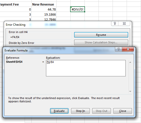
(Evaluate step 1)

In this example, F4 is divided by E4. Notice that F4 is underlined. This is the first step for the formula. It pulls the value from the referenced cell. Notice that you can step into the formula at this point, because the "Step In" button is now active. Click the "Step In" button to see the first step in the calculation.

(Step Into step 1)

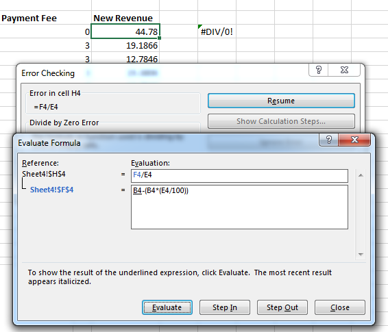
The first step into the formula references the F4 cell that also contains a formula. This formula is shown in a new text box created under the original formula text box. You can also see that a tree formation reference list shows that the cell shown in the text box is the F4 cell.

Because the original formula references a second cell that also has a formula, notice that the first cell in the formula - B4 - is underlined. The next step is to now step into this cell and retrieve its value. Click the "Step In" button again to retrieve the B4 cell value.

(Evaluation Step Into Step 2)

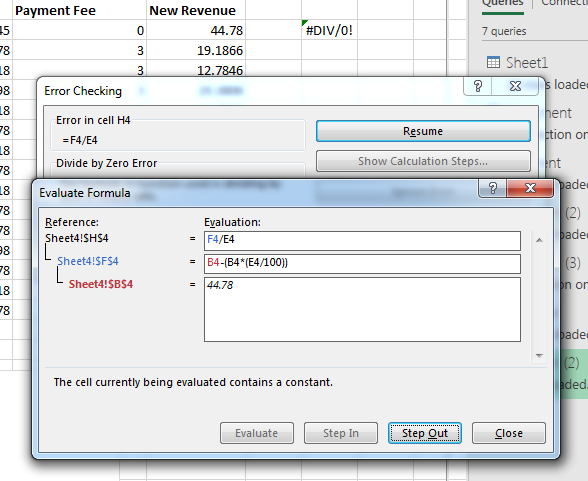
Notice that not only does Excel retrieve the B4 value, but it also calculates the formula from the previous step. The next step shows the value "44.78" and shown in the third text box. The left side of the text box identifies the value's cell name, which is B4. The previous step has B4 in red, and the label is also in red. It's the same with the blue label matching the first F4 cell reference. The color prompts show you which cell matches the value in each text box.

With the F4 cell value evaluated, you now know that the value is 44.78, so you can step out of the first cell evaluation and move on to the next cell in the main formula, which is E4. Click the "Step Out" button to move to the next cell in the calculation.

After clicking "Step Out," you'll notice that there is another cell reference in the second step, so instead of moving to E4, Excel moves to the next B4 cell. This is because Excel 2019 will step through each cell reference in the tree of values until it finds a value. The F4 cell reference three more cells, so those cells are first evaluated before you move on to the E4 cell in the main formula.

(Evaluation Step Into Step 3)

If you click "Step In" again, and the next text box shows the B4 value again. You already know that the B4 cell contains the value 44.78 from the last B4 step. It also displays now in the second text box. For each cell reference that's evaluated, the value replaces the cell reference in the text box.

Click "Step Out" after B4 is evaluated again, and then click "Step Out" to move to the next cell in the sub-formula.

 

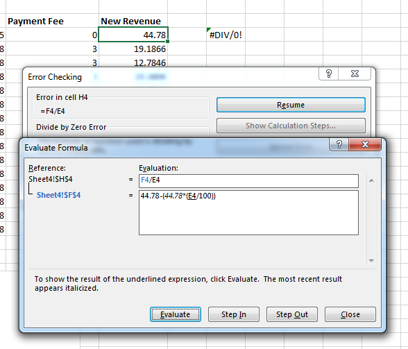
(Evaluation Step Into Step 4)

The next cell is the E4 cell. You might notice that E4 is also the reference in the main formula. Click "Step In" again and Excel 2019 evaluates the E4 cell. This cell contains the value 0, so you see "0" replace the cell reference and now all reference cells have been evaluated and replaced.

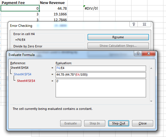
(Evaluation Step Into Step 5)

Since evaluating the E4 cell in the inner formula was the last step, the "Step In" button is disabled and now the "Step Out" button is the only one enabled. Stepping out will return you to the previous formula, which is the main one. If you have numerous inner formulas, you would have to step into and step out multiple times until your follow the steps Excel takes to calculate values to the end. Performing these steps will help you identify where in the calculation causes issues and throws an error.

Click "Step Out" and move to the E4 cell in the main formula. You know from the previous inner formula that E4, but you can click "Step In" one more time to see the value associated with the E4 cell.

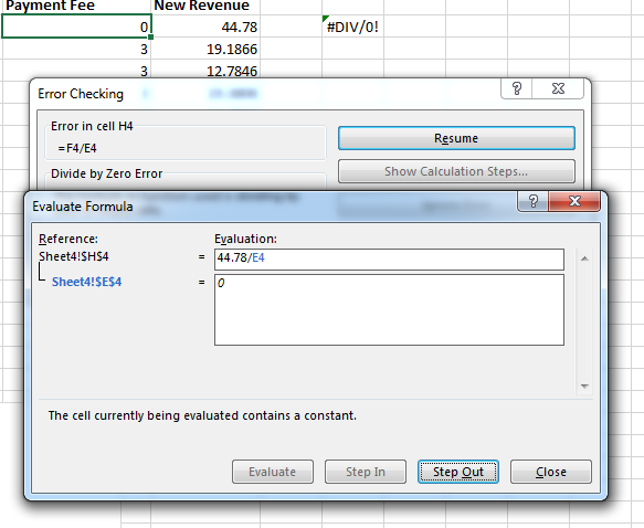
(Evaluation Step In Step 6)

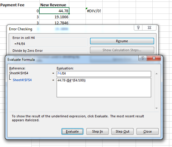
From here, you should be able to identify the issue. If at any point in this evaluation an error occurs, Excel with throw an error and stop the process. However, this error happens at the very end of the evaluation, so after clicking "Step Out," no more steps can be made and now on the "Evaluate" button is enabled.

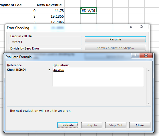
(Final evaluation)

At this point, the evaluation will calculate the formula. You know that it will result in an error, but if you didn't know where the error occurs, the evaluation tool will show you that the result of dividing 44.78 by zero will throw an error. Here is where you know that the calculate fails, and you must make changes to your data to ensure that the value is not set to 0.

Excel's auditing and troubleshooting tools will help you find errors in your formulas. For small spreadsheets, you might be able to find errors quickly from a short review, but when you have dozens of formulas across multiple worksheets, Excel's tools will help you find issues and save time in your troubleshooting.