The Most Useful And Overlooked Functions in Excel 2019

Depending on your need, Excel 2019 has several functions that automatically calculate more difficult math formulas instead of making you create your own. leaving you with the likelihood that you could make a human error when setting up your spreadsheets. This article covers some of the other useful functions that you might need should you create your own spreadsheets or work with financial and statistical spreadsheets.

Conditional Functions

Conditional statements can be used to display data depending on other data, static or dynamic. Conditional statements in Excel include "if," "and," "or," and "not." Each one of these functions represent a different logical expression that can be used to display conditional data.

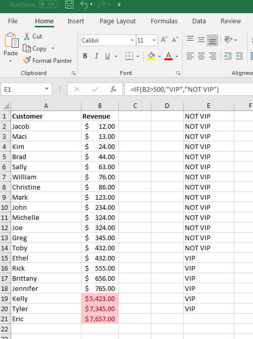
In the next examples, we'll use this data shown in the image below:

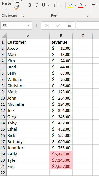
(Test data representing revenue from customers)

Test data represents fictional customers and revenue made by those customers. Remember that you don't need to memorize these formulas and functions. You can click the function lookup button to find the function that you want to use, and then get a quick view of the parameters and syntax needed for the function to work properly.

The "if" statement tells Excel to display data based on "if" a value meets a certain condition. This conditional statement is probably the most commonly used condition in Excel, so this section focuses on "IF" but the features and syntax can be used for other conditional statements in Excel 2019.

Suppose you want to display VIP customers based on revenue earned. You can use the "if" statement to display "VIP" in a cell based on the amount shown in the revenue column. We'll use the E column to display results for each function. Click the E1 cell and then click the function button to open the "find" window. Double-click the "IF" selection to open a window that asks for function arguments.

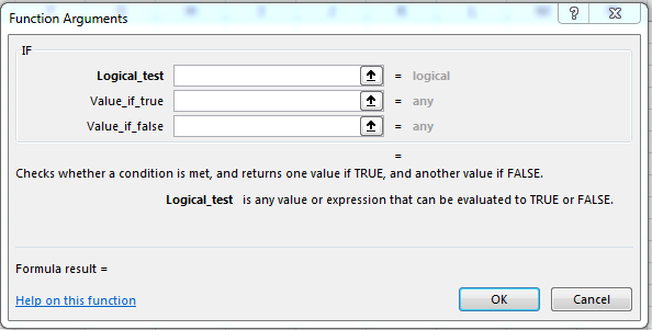
(Function arguments configuration window)

Notice that the first option is the "logical test" parameter. We want to set VIP status for any customer that provided revenue over $500. You can click the input button (up arrow icon) or type in a value. In this example, we typed B2>500, which means that you want to test if the value in B2 is greater than 500.

The next two input text boxes are what you want to show when the logical test returns true or false. If the value in B2 is greater than 500, the function returns true. Enter VIP for this result. If B2 is not greater than 500, the function returns false. You can show alternative wording should the function return false. In this example, we'll use "NOT VIP" as the wording for a false return.

When you are done, click the "OK" button to apply changes. When you create these formulas, only one cell is evaluated. The result is shown in E1.

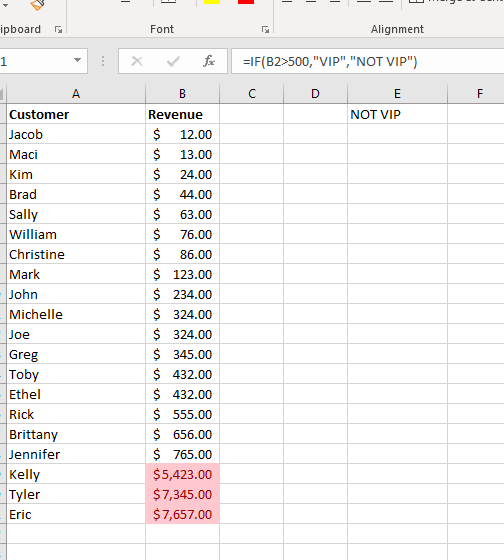
(Results from the IF function)

We want more than just one customer evaluated. We want Excel to display these results along each row. Note that we have results in E1, and normally you would have these results in E2 and flow down each row, but for simplicity we are using the top cell.

Excel has a feature named "Fill Down" that copies cell content to each row. When you have formulas as cell content, Excel 2019 evaluates the pattern and automatically changes the cells used in the formula (in this case B2) and changes the cells to represent the next row down.

Highlight E1 and then cells that span down to E20. The "Fill" button is found in the "Home" ribbon tab in the "Editing" section.

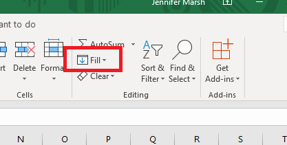
(Fill button location)

Interested in learning more? Why not take an online Excel 2021 course?

With the original cell that contains the formula selected along with the cells that you want to copy to selected, click the "Fill" button. Click "Down," but notice that you can copy in each direction along rows and columns in Excel. Excel 2019 will automatically identify that the row number must be incremented by one as it copies values. The result is a list of cells that tells you which customers are VIP.

(Fill down action based on IF formula)

If you want to match cells next to the customer row, click E1 and then select "insert." Choose "Shift cells down" and Excel recalculates the formulas and moves data down and in the same row as customer records.

Date and Time

Just like numerical values, you need a way to work with date and time values. Date and time values are critical for most reports, and Excel has several functions that work with these values. You can add values such as adding 30 days to a date. You can also extract values from a date and use it to display information. For instance, you might have a date but want to use the month to calculate values. You can extract month, day or year from a date and display it or use it in your calculations.

One of the most commonly used date and time functions is "now." The now function gets the date and time and displays it in the selected cell. This function takes no parameters, so it's one of the easiest to use in Excel.

To test this function, click any cell in a spreadsheet. Then type the following text in the cell:

=NOW()

After you press "Enter," Excel 2019 shows the result in the cell. The date and time Excel uses is from the local computer.

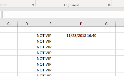
(The result of the NOW function)

You'll notice that the time uses the 24 hour military standard, but you can change the format to display it the way you want. If you recall, we discussed the way you can format numbers and other values in an Excel cell, and this includes dates. In most business applications, you want to see the date in time in standard notation, but you can also strip the time from cell content. You can do this using the format options from the number dropdown in the "Home" ribbon tab.

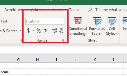
(Format option dropdown)

In the dropdown, you'll notice several date format options. You can strip the date and show only the time. You can show a long or short date. In this example, we'll display only the short date. Click the cell that contains the date, and then click the dropdown. Select "Short Date" and notice that the value displayed from the "Now" function displays only the month, day and year in the cell.

Excel also has YEAR, MONTH and DAY functions to take a part of the date. In this example, we'll show only the year in the cell. In the F3 cell, type the following content:

=YEAR(NOW())

Notice that the NOW function is used as a parameter in the YEAR function. You can use functions within functions as parameters to make your formulas more complex but get what you need from only once cell. The example above will only show the year in the F3 cell, so you can strip integer values from more complex functions.

Text Functions

Excel 2019 has several different functions that work with text. You can take parts of texts, use a FIND function to get location of string patterns, substitute values and get the length of a string. This section covers the most common text functions you'll use in Excel spreadsheets.

The concatenation function (CONCAT) combines two strings and displays the results. For instance, you might have a table of data from Access imported into Excel. Usually, a database has a first name and last name column. You might want to combine these two columns into one cell that displays a customer's first and last name. You can use the CONCAT function for this reason.

Click the function button to open a search window. Type "concat" in the search, and double click the "concat" result to open a configuration window.

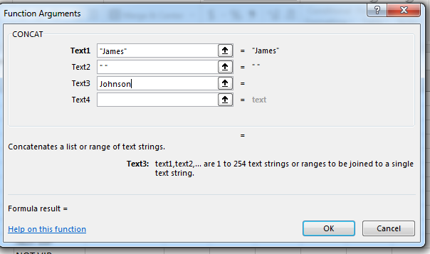
(The CONCAT function parameters)

Notice in the image above that three input parameters are used. The middle one has the space that you need between the first and last name. You can also use cell values, but for simplicity static values are shown to illustrate the way the CONCAT function works.

The result shows "James Johnson" in the selected cell.

The LEN (length) function shows the length of the text in a cell. Length returns an integer value that you can use for other reasons in your reports such as formatting based on the length of the largest word in a column.

Click the function button again and type "len" to find the length function. Double click the "LEN" option to open the configuration window.

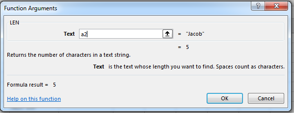
(LEN configuration window)

In the image above, the text we refer to is in the A2 cell. Excel gives you a preview of what's in the cell. In this case, "Jacob" is stored in that cell and the length returned is "5." Click "OK" and the cell selected shows the length of the cell value in A2. Should you decide to run a LEN function on the entire set of customers in the revenue spreadsheet, you can again use the "Fill Down" feature to run LEN on all rows.

The final common function is the FIND function. This function searches a string for a set parameter value and gives you the location of the pattern found if it is found. If it's not found, the FIND function returns 0.

In this next example, we'll use the FIND function to search for a text pattern in the A2 cell. We know that this cell contains the text "Jacob," so we'll find the string "cob" in this word. We know this value is found at position three, so you should expect to see the value "3" returned.

Click the function button again, and type "FIND" in the search text box. Double click the "FIND" function returned in results and you'll see the syntax window display asking for parameters.

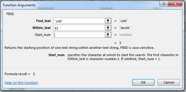
(FIND function search parameters)

In the image above, the text we're searching for is "cob" and the cell we want to search is A2. By leaving the "start" parameter blank, Excel assumes that you want to start at the first letter, but you can start the search in another location within the string.

Like other functions, a preview of the data is displayed in the window, so you know when your configurations are accurate.