If you have ever used a word processing program such as Microsoft Word before, then you are familiar with the term "outline". When you outline information in a word processing program, you organize that information by creating levels. For example, you may have a chapter on gorillas. That chapter would be a level. Then you may have sublevels on their habitat and life expectancy. Those sublevels can also have sublevels, so on, and so forth.
Outlining in Excel 2016 shares the same concept. You can outline data in a worksheet by assigning rows in the worksheet to different levels. You can then hide or display those levels. In Excel, outlining gives you the ability to organize large amounts of data.
Excel 2016 offers you three ways to create an outline:
1. Insert automatic subtotals
2. Automatically
3. Manually
We will discuss all three methods to outlining your data in this article.
Once you have outlined your data, you will see the outline symbols appear to the left side of the worksheet. To display the various levels, you will click the mouse on various symbols, as you will learn in just a few minutes.
About Outlines
There are a few things you need to know about outlines before we show you how to create and use them in your Excel worksheets. We have listed these things below. Please take the time to learn them, because these are the "rules" you will need to know when you choose to create outlines.
1. A worksheet can only contain one outline.
2. Outlines can either be created manually or automatically.
3. An outline can be created for an entire worksheet or just for a range of data.
4. You can hide the outline symbols without removing the outline. Simply press CTRL+8 to toggle the symbols off and on.
5. You can have up to eight nested levels in one outline.
Creating an Outline Automatically
Outlining groups sections of the sheet together so you can hide them.
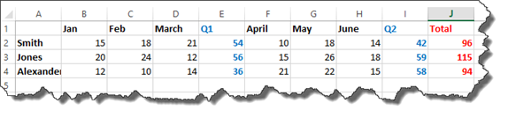
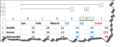
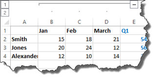
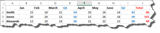
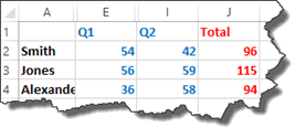
Below we have a worksheet that contains sales amounts for different employees in different months. It also contains quarterly totals, then a grand total.
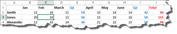
To automatically create an outline in Excel 2016, move your cursor anywhere in the data. You can see our cursor below.
Click on the Data tab.
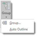
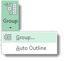
Go to the Outline group. Click the downward arrow below the Groups button, then choose Auto Outline.
As long as you have subtotals in your worksheet, it will become outlined, as shown below:
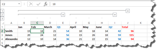
As we said at the beginning of the section, outlining groups sections of a sheet together so you can hide them if you want.
In our outline, you can see 1, 2, and 3 in the row headings. These are your outline symbols.

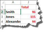
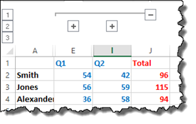
If we click 1, all the columns but the Total column is hidden.
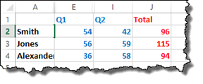
If we click 2, we see our quarterly totals along with our Total column.
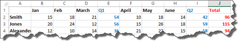
If we click 3, we see nothing is hidden.
You can also use the plus and minus signs in the outline to expand or collapse data.
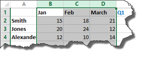
If we click 2 again, we see this:
We can click on the plus sign above column E, which represents the Q1 total to see all the data for Q1.
If you want to hide that data again, click on the minus sign in the outline above column E.
Manually Creating an Outline
In the last section, we learned how to let Excel do all the work in creating an outline. Now let's learn how to create one manually. This will be important to know if you do not have sums (or totals as in the last section) in your worksheet, which are required to create outlines automatically.
To start with, select the data you want to include in the outline, as we have done below.
Next, click on the Data tab. Go to Group, then select Group from the dropdown menu.
This groups columns of data together.
You will then see the outline symbols above the group. You can now expand and collapse to show and hide the data in the outline.
Inserting One Level of Subtotals
You can have Excel automatically calculate subtotals for a column in a list using the Outline command as well. However, you cannot do this with tables. If your data is in a table, you will first need to convert it to a normal range of data.
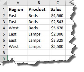
We are going to insert a subtotal for the data pictured below.
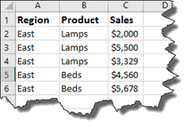
We want to have Excel automatically insert a subtotal for each product listed. To do this, the first thing we are going to do is sort the data by the product so that the products are grouped together. We need all lamp sales listed together, all bed sales, etc.
Next, we need to conduct a few quick checks of our data. We are going to do is make sure that the column we want to use to calculate a subtotal has a label in the first row. We are also going to make sure that we have the same type of data in the column. For example, all the data in the column labeled "Sales" represent monetary amounts. We are also going to make sure that the range of cells for which we want to calculate a subtotal does not include any blank columns or rows.
Next, click a cell in the Sales group since this is the data for which we want a subtotal.
Go to the Data tab, then the Outline group. Click the Subtotal button.
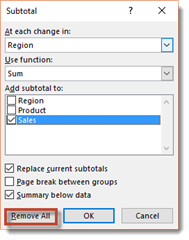
You will see the Subtotal dialogue box.

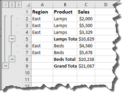
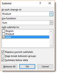
In the "At Each Change field", you will specify how to subtotal the data. We want the subtotals for each product, so we tell Excel that "at each change of product", to add up the sales for that product. This is why we choose Sum (or add) in the "Use Function" field.
In the "Add Subtotal To" field, we are going to select the column that contains the data for which we want to create a subtotal. In our example, this is the Sales column, because we want a subtotal of the sales for each product.
Click OK when you are finished.
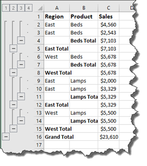
Inserting Nested Levels of Subtotals
You can also insert nested levels of subtotals.
Let's show you what we mean.
Take a look at our worksheet below.
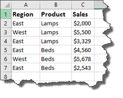
You can see that we have changed it to reflect two different regions: East and West.
We now want to create subtotals for each product sold in each region. In other words, we want a subtotal for all lamps sold in the east region, as well as the rest. The same applies to beds.
To do this, the first thing we are going to do is sort the data by the region so the regions are together, then sort by product, as shown below.
Next, we need to conduct a few quick checks of our data. We are going to do is make sure that the column we want to use to calculate a subtotal has a label in the first row. We are also going to make sure that we have the same type of data in the column. For example, all the data in the column labeled "Sales" represent monetary amounts. We are also going to make sure that the range of cells for which we want to calculate a subtotal does not include any blank columns or rows.
Select a cell in the range.
Go to the Data tab, and click the Subtotal button as you did in the last section of this article.
You will see the Subtotal dialogue box.
We want to make it so that at each change in "Region", use the Sum function to create a subtotal for the "Sales" column, as pictured below.
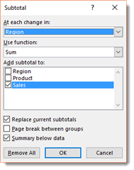
Click the OK button.
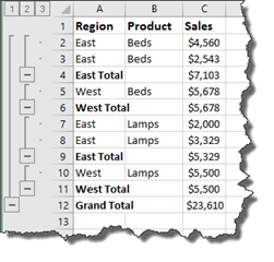
This shows the subtotal by region. However, now let's go back to the Subtotal dialogue box and select at each change in product use the sum function to add a subtotal to the sales column.

Uncheck the "Replace Current Subtotals" checkbox.
Click the OK button.
Removing Subtotals
To remove subtotals, select a cell in the data range, then go to the Data tab.
Click the Subtotal button in the Outline group.
Click Remove All in the dialogue box, as pictured below.
Hiding or Removing an Outline
As you work with your data, you may find the need to hide an outline � or to remove it completely.
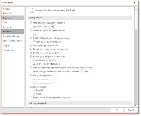
To hide an outline, go to the File tab. Click Options, then click on the Advanced tab.
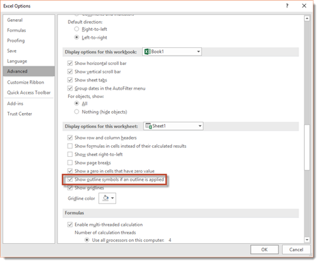
Go to the Display Options For This Worksheet section, then select the worksheet which contains the outline you want to hide.
Uncheck the box that says Show Outline Symbols If An Outline is Applied.
To remove an outline, go to the worksheet that contains the outline.
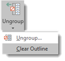
Next, go to the Data tab and go to the Outline group. Go to Ungroup, then select Clear Outline.
Editing an Outline
By using the Group and Ungroup commands under the Data tab, you can add or remove columns and rows to or from your outline.
Let's say you add a new row to your worksheet that already contains an outline.
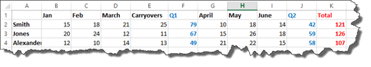
In the snapshot below, we have added a new column. We have named it Carryovers.
If this new column is not grouped with the rest of the outline, click the Data tab, then click Group and select Group.
Make sure you click on all the outline views (1, 2, and 3) to make sure that the new column is hidden when it is supposed to be. For example, if it is not hidden in 2 and it is supposed to be, you will have to go to Group under the Data tab, then select Group.
To remove a row or column and exclude it from the outline, go to the Data tab, select Ungroup, then click Ungroup.
Working with Custom Views
Custom views allow you to save display settings. For example, you can save column widths, row heights, cell selections, window settings, filter settings, and hidden rows and columns. You can also save print settings. These include headers, footers, margins, sheet, and page settings. When you save these settings in a custom view, you can easily and quickly apply them to a worksheet.
You can create different custom views for each worksheet; however, you can only apply a custom view to the worksheet that was active when the custom view was created.
Creating a Custom View
To create a custom view, first change the settings that you want to save in a custom view. We are going select a non-contiguous range of cells, as shown below.
Next, click on the View tab. Go to the Worksheet Views group, then click on Custom Views.
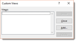
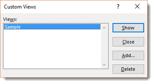
You will see the Custom Views dialogue box, as shown below.
Click the Add button.
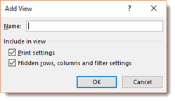
Enter a name for the view in the Name box.
Now go to Include In View and select the settings that you want to include.
Click OK.
To apply a custom view, click the View tab again, then click Custom Views. Select the name of your view in the Custom Views dialogue box.
Click the Show button.
When you click the show button, the worksheet that was active when you created the view will be displayed.
Editing and Deleting Custom Views
To edit a custom view, display the custom view you want to edit by going to View>Custom Views, selecting your custom view, then clicking the Show button. Make any changes to the view that you want to make.
Go to View>Custom Views again. Click the Add button.
Re-enter the name of the custom view that you just edited.
You will see this warning:
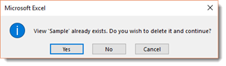
Click the Yes button.
The custom view has been edited. It will be appear with your other custom views.
To delete a custom view, go to the View tab, click Custom Views, then select the name of the custom view you want to delete. Click the Delete button.
Using an Outline to Create a Custom View
Outlines can be used to help you create custom views. You can use an outline to show or hide rows and columns. You can then create a custom view that has rows or columns hidden by using the outline.
Let's show you what we mean.
Here is our worksheet.
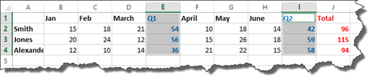
We are going to click the number 2 in our outline to hide all the data except for the columns that contain sums.
Now, we can go to View>Custom Views and save this as a custom view.
We will name the custom view Totals.
Whenever we show the custom view "Totals," we will see our worksheet as it is displayed below.
Getting Quick Access to Custom Views
You can also add custom views to the Quick Access Toolbar so that you can access them quicker and easier than going through the steps of clicking on the View tab.
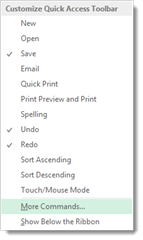
To do this, go to the Quick Access Toolbar and select More Commands.
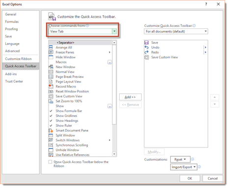
In the Choose Commands From dropdown menu, choose View Tab, as circled in red below.
Click on Save Custom View to select it.
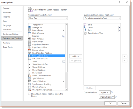
Next, click the Add button, then click OK.
You will then see a Custom Views icon displayed in the Quick Access Toolbar.

Clicking this icon will bring up the Custom Views dialogue box where you can show, add, edit, or delete custom views.
Using Excel Templates
A template is a model of a worksheet or workbook that you can customize and use as your own worksheet or workbook. Excel 2016 offers you access to a wide variety of templates that you can use to create worksheets and workbooks.
In Excel, a pre-designed template comes as a workbook. It may contain formatting, design, and layout. It may also include tables, column headers, row headers, pre-designed tables, as well as pre-designed lists. There are different types of templates for different types of workbooks and worksheets. For example, you can choose a Budget or Inventory template.
To access Excel's templates, click the File tab, then select New.
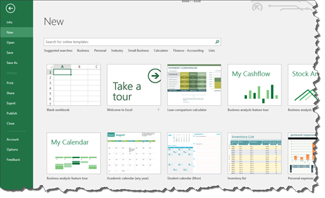
Excel offers hundreds of templates, so searching for the one you want to use may seem overwhelming. However, it does not have to be. There are several ways to search for the type of template you want.
You can type in the type of template you want into the search box.
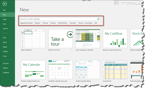
Enter keywords that will help Excel find exactly what you need. For example, you might type "invoice" or "expenses."
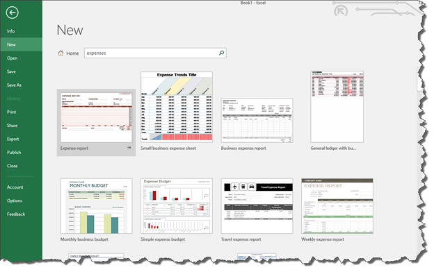
Below you can see the search results for "expenses".
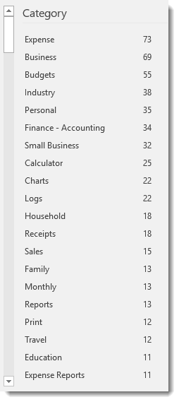
Click on a category to the right of the templates to further refine your search.
To open a template, click on it.
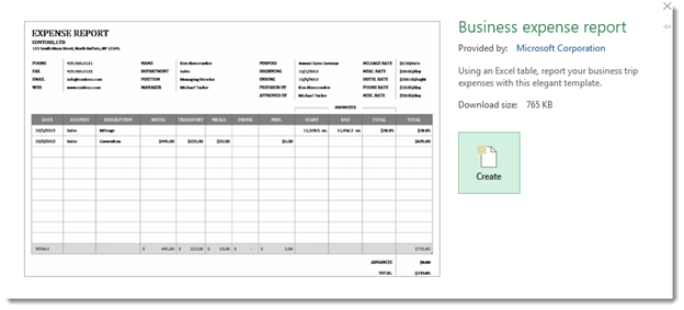
Click the Create button.
You should already be familiar with templates, as well as how to open an Excel 2016 pre-designed template. However, take the time to explore the multitude of pre-designed templates available to you.
Creating a Template
In addition to using a pre-designed template, Excel gives you the ability to create your own as well.
Templates can be helpful to create if you want to create a universal look for all of your workbooks and worksheets. For example, if you do invoicing for your company using Excel, creating an invoicing template with your company's logo, name, and address can save a lot of time over adding those things each time you create an invoice. In addition, you can also add the rows and columns that you want to appear in your template.
In summary, you can save the following things in a template:
-
Text including page titles, row labels, and column labels.
-
Data, such as constant values that includes tax rates, profit margins, and contact information.
-
Graphics, such a logo (as we mentioned above).
-
Formulas that you will use on future sheets, such as sums and averages.
To create your own template, all you have to do is design your workbook. It may contain several worksheets or just one. Use the Insert tab to add graphics. Add row and column labels, data, any formulas (such as with a Total box for an invoice).
You can also customize the appearance by going to the Page Layout tab and choosing a theme and adding a background image.
Take time to format the text and data as well.
In the example below, we have started to create a template.
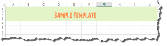
We started by adding a fill color to a selected range of cells by going to the Home tab and clicking the Fill Color button:  .
.
Next, we clicked the Insert tab and inserted an image. We double clicked on the image to remove the background.
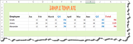
Next, we added row and column headers.
We already added our formulas earlier in this article.
Under the Page Layout tab, we selected a theme, specified our margins, and also chose to have the gridlines printed.

We also set our print area by selecting the area, then going to Print Area>Set Print Area.
If your spreadsheet is wide, you will also want to set the scale so the entire worksheet prints, as well as the orientation.
When creating your own template, you should go ahead and apply all the settings that you want applied to every workbook and/or worksheet that uses this template.
Take the time to create your template.
When you are finished, go to File>Save As.
Choose the location where you want to store the template.
Then, enter a name for the file in the File Name text box.
Choose Excel Template (*.xlts) from the Save as Type dropdown menu.
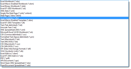
Click the Save button.