Data Validation in Excel 2016

Data validation in Excel allows you to define what type of data should be entered into a cell and allows you to prevent invalid data from being entered. In addition, you can create messages that will tell users what type of data should be entered into a specified cell, then provide instructions for correct input.

For example, you can restrict the number of characters permitted in a cell. If you have a column that is for zip codes, you can restrict the number of characters to five to prevent typos and other errors.

Entering Data Validation Criteria

In order to make data validation work, you have to tell Excel what type of data you want to allow in a cell or range of cells. In other words, you have to create criteria that must be met in order for the data to be permitted.

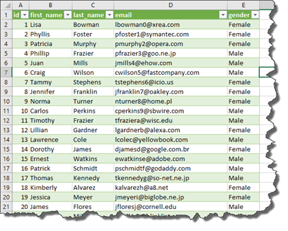
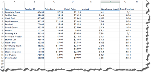
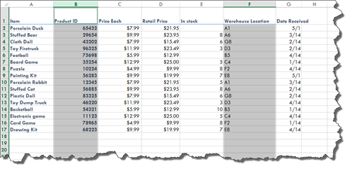
Take a look at our worksheet below.

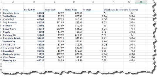
In our PRODUCT ID column, all of our product IDs contain five characters. This is because all of our fictional product IDs are exactly five characters long. In addition, they are only numbers. There are no letters.

We want to prohibit any more than five characters being entered into these cells. What is more, we want to prevent letters from being added.

To do this, we are going to select the column we want to apply these restrictions to.

Next, we go to the Data tab then go to Data Validation dropdown arrow, and select Data Validation.

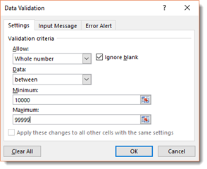
We have already entered our criteria in this box; however, let's review it.

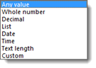
Click the Allow dropdown menu. Choose the type of data that you want to ALLOW in the cell or range of cells.

We chose whole number. We also left the checkmark in the Ignore Blank box, because it is okay for a cell to be left blank.

Next, choose the range for your data from the Data dropdown menu.

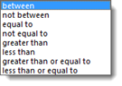
These options should all be familiar to you, so you should understand how they will work to restrict the types of data that can be entered.

For our example, we have chosen between, so we are then asked to enter the lowest number we will accept, then the highest number.

Click OK.

Now we can try to enter data into the column that does not meet the criteria.

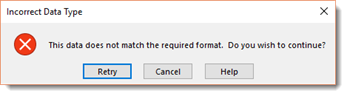
We are met with this message:

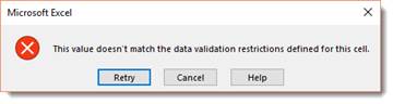
We can choose to Retry and enter the data again, cancel and not enter the data, or get Help.

Adding Input Messages

An input message is a message that appears whenever a cell that contains data validation rules is selected.

An example is shown below.

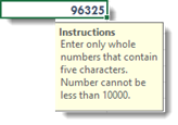
You create input messages to let anyone who enters data into your worksheet know what specific type of data can be entered into the active cell. This clues them in, so to speak, so they can enter the type of data that is requested.

To enter an input message, go to the Data tab again, then go to Data Validation. Select Data Validation.

You will be brought back to the Data Validation dialogue box.

Click the Input Message tab.

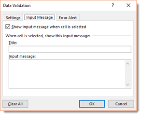
Whenever the cell is selected, you want the message to appear, so leave the checkmark beside the box Show Input Message When Cell is Selected.

Next, enter the title for your message. We are going to enter "Instructions."

In the Input Message field, enter the message you want to be displayed.

You can see ours below.

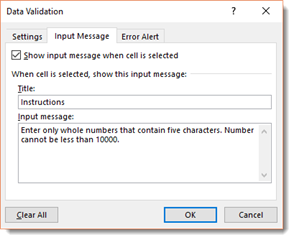
Click the OK button.

Now, whenever a user clicks on a cell that contains the data rules we specified in the last section, they will be met with this message:

Customizing the Error Message

As we saw earlier in this article, when someone enters an incorrect type of data into a cell where you have placed data rules, they are met with this default message:

You can customize this message to provide instructions so that the user will be more likely to press Retry.

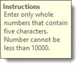
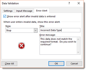
To do this, go to the Data tab. Click on the dropdown arrow for Data Validation, then select Data Validation. Click the Error Alert tab.

Leave the checkmark in place, because you want the error message displayed so a user knows they have entered an incorrect type of data.

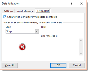
Next, choose a style from the dropdown menu. STOP is chosen by default. We are going to choose Warning.

Let's review the three types of styles you can choose.

Stop gives the user a chance to reenter the data.
Warning allows the user to enter the incorrect type of data anyway by clicking YES. They can click NO if they do not want to enter it.
Instructions provides the same options as warning, except it is an information icon instead of a warning icon.

Next, enter a title for the message, then the message you want to appear, as we have done below.

Since ours is a warning, we want to ask them a YES/NO question.

Click OK.

This is our new error message:

Locating Invalid Data within a Data Validation Range

As you saw in the last section, if you set your error message to the styles Warning or Information, users are still allowed to enter invalid data. They just have to confirm that they want to enter it.

In our worksheet below, we have invalid data that has been entered into our PRODUCT ID column.

What we now want to do is to be able to find the invalid data.

To find the invalid data, go to the Data tab. Select Data Validation>Circle Invalid Data.

Look at what happens in our worksheet.

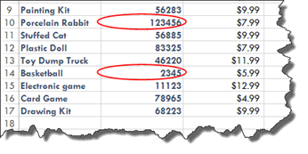
The invalid data is circled for us.

The data can now be edited so it becomes valid.

To remove the circles, go to the Data Validation dropdown menu, and select Clear Validation Circles.

Creating Data Validation Dropdown Lists

Sometimes it is a good idea to give people who enter data into your worksheet a dropdown list of data choices that they can enter into a cell.

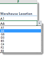
If you look at our worksheet below, you can see the column Warehouse Location.

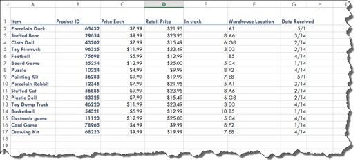
In order to prevent the wrong type of data from being entered or typos from occurring, we can create a dropdown list in each cell that gives a list of warehouse locations to choose from.

To do this, we are going to create a list of warehouse locations, as shown below.

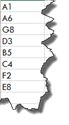
You can create this list outside of the table.

Now, we go back and select the cells in the table for which we want to create the dropdown list.

Click on the Data tab, then go to the Data Validation dropdown, and select Data Validation.

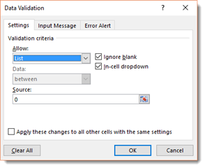
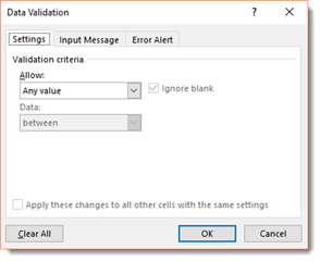
In the Data Validation dropdown box, click on the Settings tab.

We can now enter our data validation material.

From the Allow dropdown menu, choose List, as we have done below.

Next, click in the source field, then select the source for your list. This is the data in the new worksheet that we created.

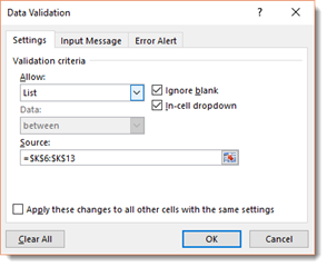
Click the OK button.

Whenever you click in one of the cells with the new set of validation rules applied, you will see a downward arrow and a dropdown list.

Locating Cells that Have Data Validation Applied

To find cells that have data validation rules applied to them, click the Home tab, then go to the Editing group.

Click the Find & Select dropdown menu.

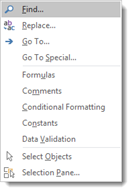
Select Go to Special.

Put a check beside Data Validation, then All, as pictured below.

Click the OK button.

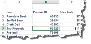
Excel then highlights all cells with data validation rules applied.

You can also find which cells contain certain data validation rules.

In our worksheet below, we have selected a cell by clicking on it. We know this cell has data validation rules applied to it. We want to find what cells have the same rules.

Go back to the Home tab.

Choose Go to Special from the Find & Select dropdown list.

This time, put a check beside Data Validation, then Same.

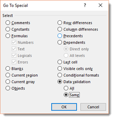
Click the OK button.

You can then see the cells that have the same validation rules as the selected cell.

Clearing Validation Rules

If you want to clear validation rules from a cell or range of cells, select the cells, then go to the Data tab.

Click the Data Validation dropdown arrow, then select Data Validation.

You will then see the Data Validation dialogue box.

Click the Clear All button.

Using Get & Transform to Perform Queries

We focused on importing data from text files, Access files, and the web. That said, you can also import data from other databases into Excel 2016. Get & Transform is a tool you can use to do this.

The Get & Transform tool will get – or import – your data, then transform it – or refine it -- for you. The neat thing about this tool, though, is you only have to "refine" the data that you import once. For example, let's say you import a weekly report from your company's database. The first time you import the data, you will have to spend the time transforming it – or refine it. After that first time, however, Excel will remember what steps you took to transform the data, and it will do it for you after that.

Data Source Options

Let's take a look at the types of data that you can retrieve using the Get & Transform tool. To see the types of data, go to the Data tab, then the Get & Transform group. Click on New Query.

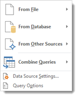
As you can see in the snapshots above, your data sources include files, databases, and other sources such as web pages.

You will see the Navigator dialogue box whenever you select a source. It will show you all the tables available. It will also show you a preview of the selected table. If you want to work with that table, you will click Load. You will then be able to work with that table in the Query Editor.

Using Another Excel Workbook as a Data Source

You can use another Excel workbook as your data source. The workbook does not need to be open for you to do this. Since this is a simple query to do, we are going to start with this before moving on to more complex queries.

To use another Excel workbook as a data source, go to the Data tab, then the Get & Transform group.

Click the New Query dropdown, then select File. Choose From Workbook.

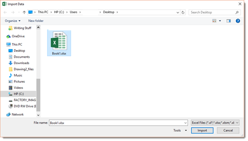
Locate the Excel workbook, then click the Import button.

You will then see the Navigator dialogue box, as pictured below.

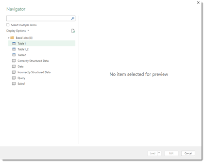
As you can see above, the Navigator dialogue box shows you all tables and worksheets in your workbook. These appear on the left.

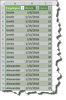
Select a table in your workbook, and it will appear in the preview area on the right.

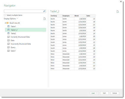
Once you select the table that you want to work with, click the Edit button.

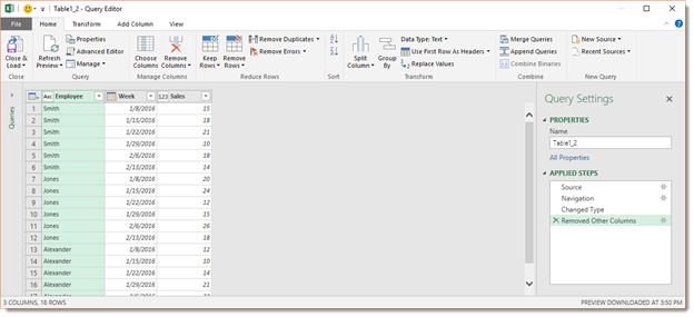
This loads the Query Editor. The Query Editor is where you will manipulate the data that will be returned to Excel 2016.

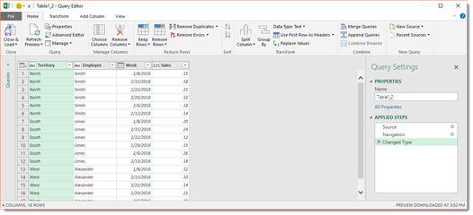
In other words, you will use the Query Editor to edit the data before you import it into Excel.

Let's say we want to remove the Territory column.

Click the Home tab in the Query Editor. Go to Choose Columns in the Manage Columns group.

You will then see all your columns listed, as shown below.

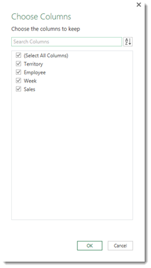
Click the remove the checkmark beside the Territory column.

Click the OK button.

The column is now removed.

Taking a Look at the Applied Steps

Earlier in this article, we told you that when you performed a query and transformed the data, that Excel would remember the steps you took to transform the data.

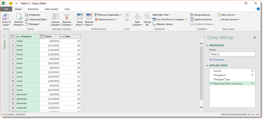
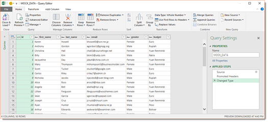
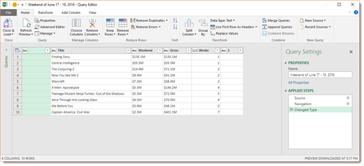
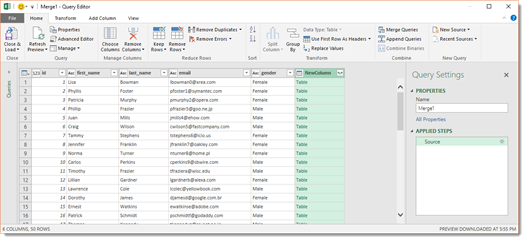
Take a look at the Query Settings pane that is located on the right side of the Query Editor.

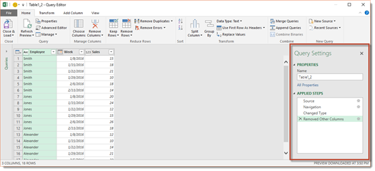
In the Query Settings pane, you can see Applied Steps. Whenever you perform a "step", it is listed in the Applied Steps field.

You can see the steps that we performed listed there. "Source" is when we chose the source file. "Navigation" was choosing the table in the source file. "Change Type" is a data type change. Then, of course, we removed columns.

Importing Data into Excel

Once you are finished recording your data, click the Home tab in the Query Editor, and click on the Close & Load button. This loads your data into your current Excel workbook and onto a new Excel worksheet.

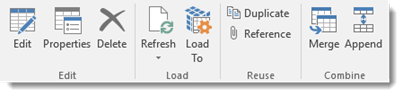
Notice that when the table is still selected in Excel, two new tabs appear in the Ribbon.

These tabs are the Table Tools Design tab and the Query Tools Query tab.

Modifying a Query

Now that the data is imported and loaded into our Excel workbook, we are going to modify the query. To do this, we are going to go to the Query Tools Query tab. This tab is pictured below.

Go to the Edit group, then click the Edit button.

This brings up the Query Editor.

Click the Add Column tab in the Query Editor, then choose Add Custom Column in the General group.

Give the new column a name.

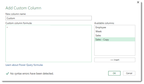
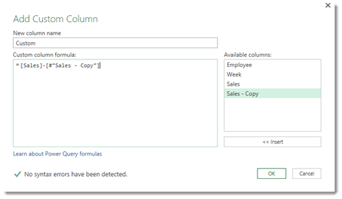
Want to learn more? Take an online course in Advanced Excel 2016.

Enter a formula to create the data for each row in the new column. Perhaps you want the difference between two of the columns, or the sum of the two columns.

To enter the formula, click on a column name from the right, then click Insert.

Enter a mathematical operator, then click another column from the right, and click Insert.

If you mess up and need to start over, just click the "X" beside the step that you messed up in the Applied Steps box in the Query Settings pane.

Refreshing Queries

You can refresh a query by going to the Query Tools Query tab. Click Refresh in the Load group.

Summarizing Data

Now let's learn to perform a query and get Excel to perform a summary of the data for us. To do this, we are going to use source data in a CSV file.

Open a new workbook, then go to the Data tab. In the Get & Transform group, select New Query, then choose From File, then from CSV.

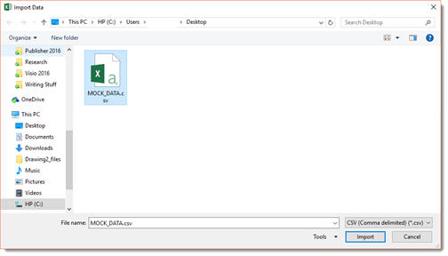
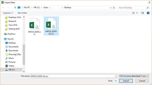
Select the CSV file you want to use, then click the Import button.

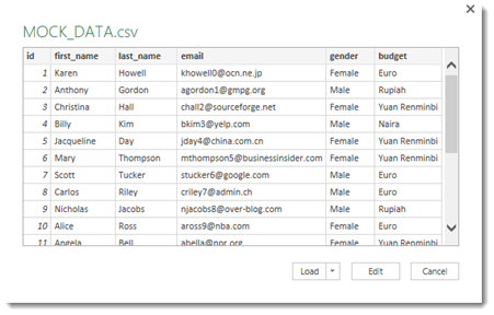
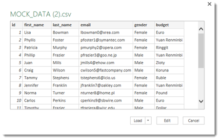
The data in our CSV file is shown above in the Navigator window.

Click the Edit button to load the Query Editor.

When you summarize data, you create groups of rows. To do this, click the Transform tab in the Query Editor. Click Group By in the Table group.

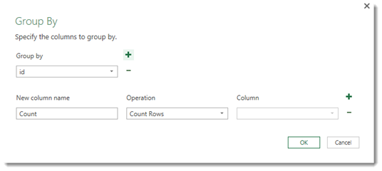
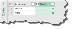
In the Group By field, we are going to select what column header we want to group by. We are going to select Gender. We want to know how many males and how many females are listed in our data.

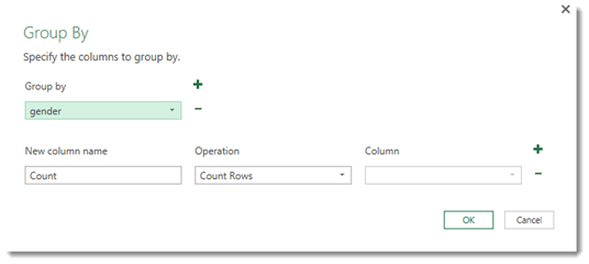
In the New Column Name field, enter a name for the new column. We are going to leave it at Count since we want to count the number of males and females.

We are also going to leave the Operation field as Count Rows as well.

Now we can click the OK button.

As you can see below, Excel summarizes our data for us, and tells us how many males and females are listed in our data.

Click the Home tab, then the Close & Load button to load the data into Excel.

NOTE: You could have also created a Pivot table after importing the original data into Excel.

Performing a Web Query

When you perform a web query, you use a web page as your data source. To perform a web query, go to the Data tab, then click the New Query dropdown. Select From Other Sources, then From Web.

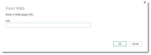
Enter in the URL of the webpage that you want to use to get your data, then click the OK button.

You will then see the Navigator window.

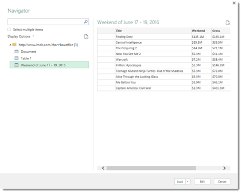
There are three items displayed for this web page on the left hand side of the Navigator window. We have chosen the third.

Click the edit button to transform the data in the Query Editor.

We want to transform the data in the Weekend and Gross columns so the actual values are displayed. To do this, we are going to click the Weekend column header, then press CTRL to also select the Gross column header.

Next, go to the Transform tab in the Query Editor. Go to the Any Column group and select Replace Values.

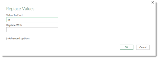
In the Values to Find field, enter M. We know that M stands for million, but we want to use actual values.

Leave the Replace With field blank, because we just want to get rid of the M.

Press the OK button.

Next, with the same two columns selected, go to the Any Column group again and select Decimal Number from the Data Type dropdown menu to convert the entries to decimal numbers.

When you are finished, select just the Weekend column header. Go to the Transform tab, then the Number Column group. Select Multiply from the Standard dropdown.

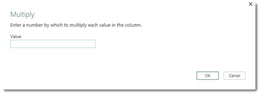
Enter in 1000000, then click the OK button.

Follow the same steps with the Gross column.

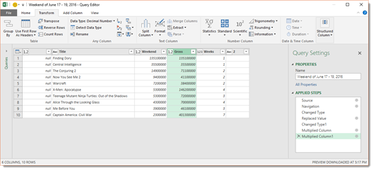
Go to the Home tab, then click the Close & Load button.

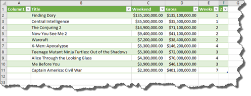
In the snapshot above, we formatted the cells in the Weekend and gross columns so the values display as currency.

Merging Web Queries

You can perform two different web queries, then merge those two queries together to produce one table of results in Excel 2016.

If you are following along with this article in Excel, open a new workbook.

We are going to start by performing the first query to retrieve data from a CSV file.

To do this, go to the Data tab, then go to the Get & Transform group.

Click the New Query dropdown, and select From File, then From CSV.

Select the CSV file for your first query, then click the Import button.

Click the Edit button to load the Query Editor.

We are going to delete the Budget column as we learned to do earlier in this article.

Let's review how to do it.

Click the Choose Columns button under the Home tab.

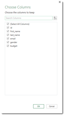
Remove the checkmark beside the column that you want to remove, then click the OK button.

When you are finished, go back to the Home tab, then click the Close & Load button.

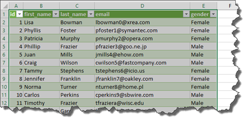
The data is then loaded into Excel.

Now let's perform the second query by creating a new worksheet in the same workbook.

Click on a cell in the new worksheet, then follow the steps above to perform another query.

We are going to use another CSV file.

Use the Query Editor to apply any transformations to your data, then load the data into Excel. We removed the Budget column from the table as we did with the first query.

We now have two queries and two tables from those queries. Since the tables have the same columns, merging these queries will be easy. Even if our tables only had one common column, merging the queries would have not been difficult.

To merge the queries, click in any cell in the first table, then go to the Data tab. Click the New Query button dropdown, then go to Combine Queries, then Merge.

You will then see the Merge dialogue box.

As you can see, each of our tables appears in the dialogue box. If one did not appear, you can select it from the dropdown.

Select the column that you will use to merge the two queries. We selected Gender.

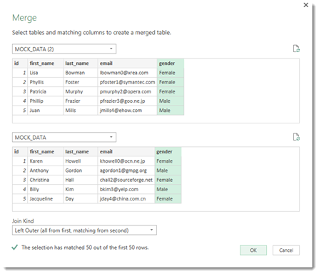
Next, select a Join Kind.

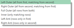
We want Left Outer. This means it will include all records from the first table, then records from the second table that have matching values. There is a description of what each join does in the dropdown menu, as shown above.

Click the OK button.

The Query Editor then opens.