PivotTables are an invaluable tool in Excel because they give you a way to summarize data; however, they also give you a way to look at the exact data that you need. Let's face it. Worksheets can contain tons of data.   You may have a worksheet that contains a list of employees, the departments they work in, their job titles, the location where they work, and their salary – and there may be 1500 employees.   By using a pivot table, you can easily view only the employees who work in the Accounting Department in your Denver, Colorado location (as an example). That said, there is so much to learn about PivotTables that we are going to continue to talk about them in this article. 

Adding Multiple Fields to Columns and Rows to a PivotTable

In all the pivot table examples thus far, we have used only one field per column or row. However, we can also add multiple fields to columns and rows.

Below is our data.

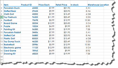
Now we are going to create a pivot table by going to the Insert tab, then clicking the PivotTable button.

We are going to place our pivot table in a new worksheet.

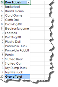
To start with, we are going to add the Item field as a row in our pivot table.

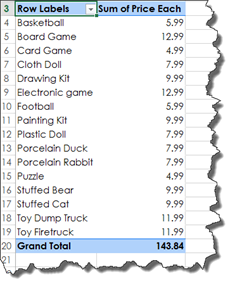
We are going to add the Price Each field to the Values section.

Now, we want to add another field to our rows.  We want to add the Product ID. To do that, we are going to drag the Product ID field to Row section and place it beneath Item.

We also want to add the warehouse location of each item, so we are going to drag that to the Row section as well.

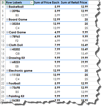
Take a look at our pivot table:

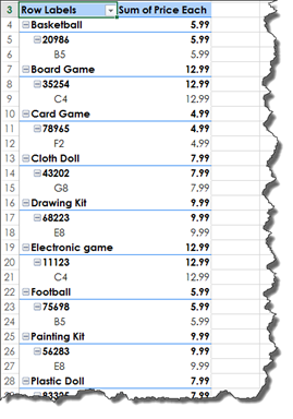
We now have Item as the heading for each row, then Product ID and Warehouse Location for subheadings.

Now, let's add another value. Let's add Retail Price.

You can add as many additional fields as you want to your rows and columns.  

Grand Totals and Subtotals in PivotTables

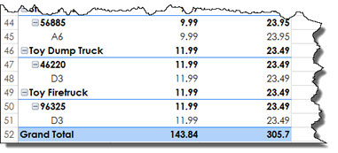
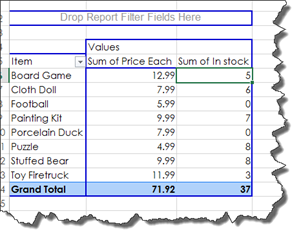
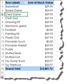
Grand totals are always displayed by default in Excel 2016. If you look at the bottom of our pivot table, you will see the grand total:

If you do not want grand totals displayed, you can turn them off by going to the Analyze tab under PivotTable tools, then Options.

Click the Totals & Filters tab.

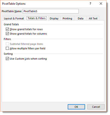
You can then uncheck Show Grand Total for Rows and/or Show Grand Totals for Columns.

Subtotals are also automatically displayed in our pivot table. 

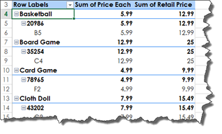
If you do not want subtotals to appear, right click on the field label. In our example above, it is Basketball. 

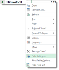
Select Field Settings.

As you can see, Subtotals are turned on by default (Automatic).

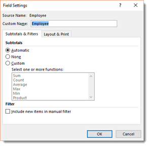
Put a check beside None, then click OK.

Of course, you can always choose to present the subtotals using a different function.   You can choose Count, Average, Product, and etc. by putting a check beside Custom, then clicking OK.

About Empty Cells in PivotTables

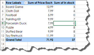
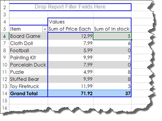
Sometimes you may see empty cells appear in your pivot table. We have highlighted such cells in our pivot table below.

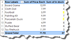
You may wish to make it so that a 0 appears in those cells rather than having them appear blank.

To do this, click anywhere in the pivot table, then right click.

Select PivotTable options, then go to the Layout & Format tab.

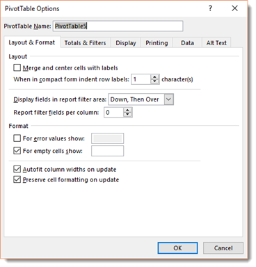
Go to the Format section.

Put a checkmark beside For Empty Cells Show, then enter a 0 in the box.

Click OK.

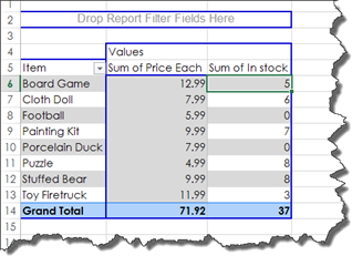
As you can see, zeros now appear in the empty cells.

Manual Grouping

You can also group things together in your pivot table.

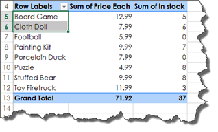
Let's say in our pivot table that we want to group together the board game and the cloth doll. 

We are going to select those.

Now, we are going to go to the Analyze tab, then click Group Selection.

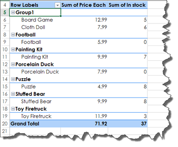
You can now see Group1 in our pivot table.  

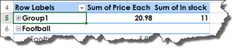
If we compress the group, it will show us a subtotal.

Take a look at our pivot table again. Notice that when we put the two items into a group, the rest of the items are listed as groups as well, even if none of them are grouped together.

To rename a group, select the group, then rename it in the Formula Bar.

Another Way to Create PivotTables

Here is another way to create PivotTables without having to drag different fields into different sections of the PivotTable Fields panel.

Go to the Analyze tab, then click Options.

Click the Display tab.

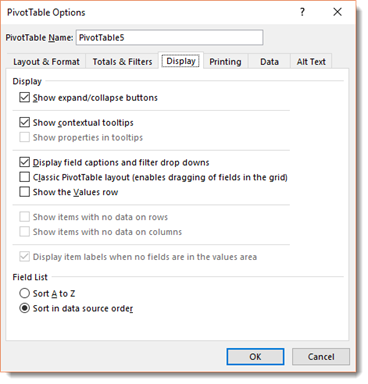
Put a checkmark beside Classic PivotTable Layout, then click OK.

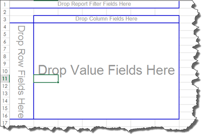
Now you can drag fields from the PivotTable Fields panel right onto your pivot table.

Working with PivotTable Styles

The PivotTable styles are found under the Design tab of the PivotTable tools. You can see this tab when you click anywhere in your pivot table. 

A style will apply formatting to your pivot table.   It can change the color, font, and other attributes.

The different pivot table styles are pictured below in the Ribbon.

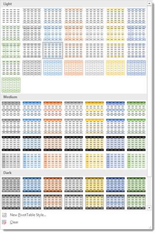
You can simply mouseover any of these styles to see how it will look when applied to your pivot table.

This is the style that we have chosen:

Based on the style that you choose, you may be able to turn row headers on or off by adding or removing the checkmark in the Ribbon.

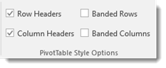
The same is true for column headers. We have chosen to turn ours off since they were on by default so that you can see the difference.

You can also choose if you want banded rows:

Or banded columns:

In addition to applying a style, we can also choose the report layout.

To do this, click the Report Layout button under the Design tab.

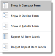
You can click on the different layouts to see how they affect your pivot table.

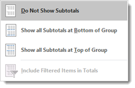
By clicking the Subtotals button under the Design tab, we can choose if and how subtotals are displayed.

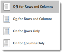
By clicking the Grand Totals button under the Design tab, we can choose our preference for how grand totals are displayed.

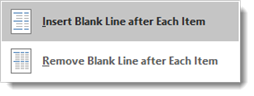
By clicking on the Blank Row button under the Design tab, we can insert blank rows to make our pivot table easier to read.

Creating a Custom PivotTable Style

If you do not want to use a built-in PivotTable style, you can create your own style using the tools provided in Excel 2016.

To do this, go to PivotTable Styles in the Design tab. Select New PivotTable Style from the dropdown menu.

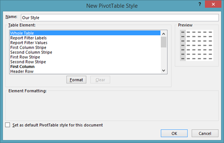
You will then see the New PivotTable Style dialogue box.

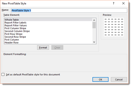
Start out by entering a name for the style.

Now what you need to do is format each aspect of the pivot table.

We are going to start with the first column. Click on First Column, as we have done below.

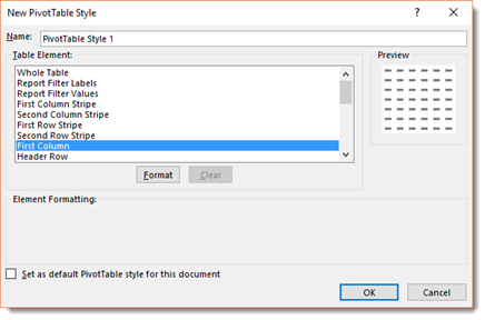
Now click the Format button.

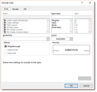
Under the font tab, set your font type, style, and size.   You can also choose your font color.

Click the Border tab.

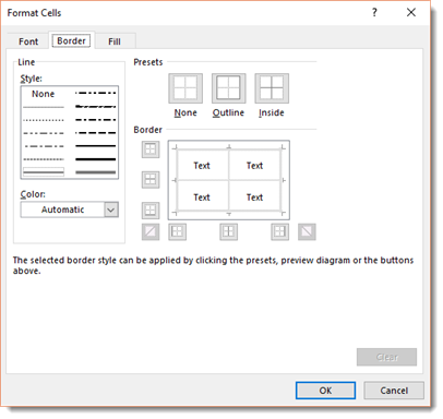
Choose the border style that you want, as well as where the border appears.

Next, click the Fill tab.

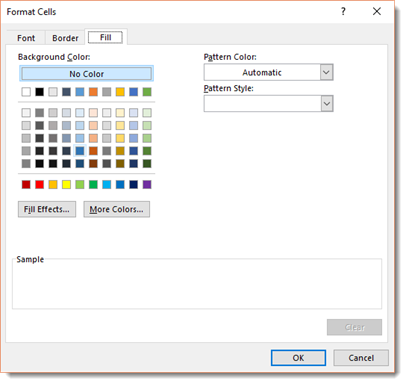
Choose a fill color for the column.

When you are finished, click the OK button.

This takes us back to the New PivotTable Style dialogue box.

First Column now appears in bold print to let us know that we have chosen formatting for it.

Now let's click on Whole Table, then click the Format button.

Follow the same steps again.   Repeat the steps until you have your new style created, then click OK in the New PivotTable Style dialogue box.

Your new style will then appear in the PivotTable Styles under the Design tab.

Click on it to apply it to your pivot table.

Creating Calculated Fields

Calculations can be done within a pivot table without having to access the original data. 

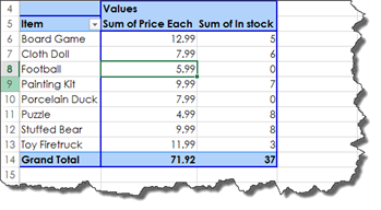
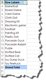
In our pivot table below, we have our items listed.   We have not added any values to the table yet, because we want to calculate the value of all the items in stock in our pivot table.

To do this, we are going to add a calculated field. Click on Fields, Items, & Sets under the Analyze tab, then select Calculated Field.

We then see the Insert Calculated Field dialogue box.

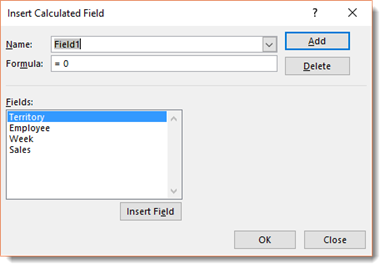
Enter a name for the field.

Next, create a formula for the field. Do so by clicking the fields from the Fields list.

We are going to select Price Each, followed by the operator for multiply, then In Stock.

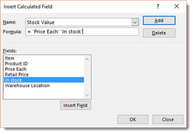
Now click OK.

The Timeline Filter Option

The timeline is new in Excel 2016. Whenever you have dates included in your original data, you can use the timeline to help further sort your data – without adding those dates to your pivot table.

Let's show you what we mean.

Take a look at our pivot table below.

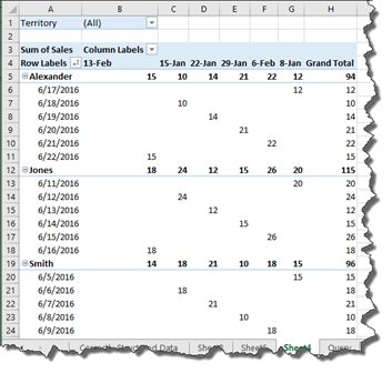
We have our sales and the date the sales were entered into the system.

We want to find out the dates on which we entered the sales.   We do not have this information as a row or column in our pivot table, but it is in our original data from which we created the pivot table.

To view the timeline and be able to filter by the dates, we are going to click in our pivot table, then go to the Analyze tab.

Click Insert Timeline.

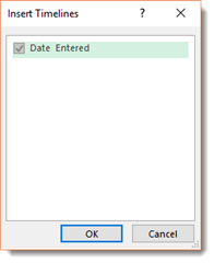
As you can see, we only have one field in our original data that contains dates, so we put a checkmark beside it, then click OK.

We can now see our timeline.

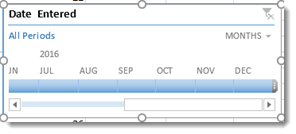
It is shown as a floating window in our worksheet.

Next, click on a month in the timeline – or select multiple months – to filter the data.

The Data Slicer

The data slicer provides another way to filter data in your pivot table. The slicer allows you to choose any fields in your data, then use that as a filter in the pivot table. You can use any of the fields in your original data to filter the data in your pivot table.

To add a slicer to a pivot table, click inside your pivot table, then click Insert Slider under the Analyze tab.

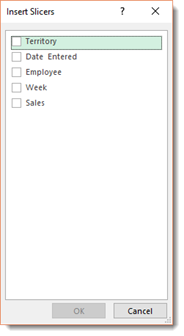
Put a checkmark beside the fields you want to use to filter the pivot table and for which you want the slicers created, then click OK.

We chose Territory.

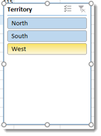
Once the slicers are created, filter the data by selecting the items you want to display in each slicer by clicking them. 

We clicked on South.

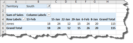
We now see our filtered results in the pivot table.

Using Data from a SQL Server

So far, we have used pivot tables that used data from the same workbook. We can also create a pivot table from an external database, such as an SQL server.

To do this, we are going to create a blank worksheet, then go to the Data tab.

Click the From Other Sources button, and select From SQL Server.

You will then see the Data Connection Wizard.

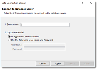
Enter your information to connect to your SQL server.

Click Next.

In the next window, you will see a list of the data available on the server.

Select that data you want to use, then click Next.

This brings you to the final window. In this window, Excel will give your data a file name. This is because Excel will save the connection if you want to use it again in the future.

Click Finish.

You will then see the Import Data dialogue box.

In the Select How You Want to Use this Data In Your Workbook section, choose PivotTable Report.

Choose if you want to place it in an existing worksheet or a new worksheet.

Now you will see your fields in the PivotTable Fields panel on the right side of your Excel window. 

You can now follow the same steps you learned earlier  to create a pivot table. However, instead of using the data from the workbook, it will use the data you have imported from your SQL server.