An Overview of What-If Analysis Methods

There are three different types of What-If Analysis tools offered in Excel: Scenarios, Goal Seek and Data Tables. This overview provides a brief explanation of all three so that you can decide which solution is best for the outcome that you're looking for.

Scenarios are probably the most common for individual users. A scenario takes data from your Excel spreadsheets and displays results based on the scenario factor. Scenarios are useful if you want to know results based on different data sets. For instance, you might want to know how much revenue you make next year based on prices of products. You can create scenarios with product different pricing data sets.

In some cases, you want to know how to get to a different goal. The Goal Seek tool helps determine what values are required to get a specific result. For instance, suppose that you have a budget each month. You don't want to go over a specific amount when you buy a new car, so you use Goal Seek to find an interest rate that matches the monthly payment that you can afford.

For each of your analysis spreadsheets, you have formulas that use data and calculate results. Formulas use variables as input and calculate based on changes in these variables. Using a Data Table, you can see the result of a formula calculation by changing one or two variables. Data Tables are useful when you want to see how data changes based on just a one-factor change in the calculation.

The examples in this overview are just a few ways that you can use a What-If Analysis spreadsheet, but these tools are used much more frequently in everyday business. Understanding these tools will help you make better decisions with finances and future purchases.

Creating a Scenario

Suppose that you want to figure out how much revenue is needed to make a specific gross profit. You can use scenarios to use different data sets. Instead of manually changing data sets or making multiple spreadsheets based on "what if" factors, you can use Excel's scenario tool.

To test this application, you first need some test data. The following image shows the test data we're using. Note that the "Profit" row is a formula that subtracts operation costs from gross revenue. The formula is shown in the content text box.

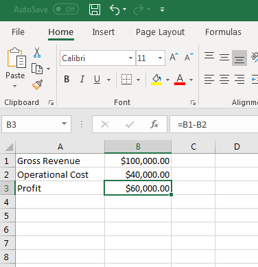
(Sample scenario data set)

Highlight all of these cells and go to the Data tab. This tab has the What-If Analysis tools that you'll need. The tool you use depends on the type of result that you want.

With the cells selected, click the "What-If Analysis" button and then click "Scenario Manager" from the dropdown list.

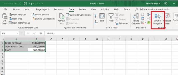
(What-If Analysis tools are in the Data tab)

A window opens where you must add a new scenario. Click "Add" to provide a name for your scenario.

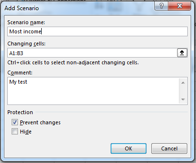
(Scenario name)

The cells you selected are already filed out in the form, but should you decide to change the cell range this is where you can change it. Provide a name for your scenario, and then check the box labeled "Prevent changes" if you don't want any changes made to the data.

A window then displays asking for static values. Since we highlight all cells that we wanted to use before opening the scenario configuration window, the values are already provided in the next window. Excel 2019 lets you know that the subtraction equation must be converted to static values, so you will need to manually calculate the result while setting up your scenarios.

Click "OK" and your new scenario displays in the Scenario Manager.

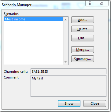
(Scenario Manager)

You just created the first scenario, but now you need another one. Repeat these steps to add another scenario. The next scenario can be the lowest income possible should costs be too high for maximum profit.

Set up another scenario using the same steps, and both show in the Scenario Manager.

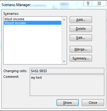
(Scenario Manager with two scenarios)

With Scenario Manager open, you can double-click the scenario name and watch the underlying data change on the opened worksheet. You can also see changes in scenario data and results by clicking the "Show" button.

Clicking "Summary" will ask for the cells where you want to review results. The "Merge" button combines several scenarios in one worksheet. This is beneficial if you have several of the same type of scenarios such as a budget for each month in individual years.

Setting Up Goal Seek Reports

A Goal Seek report is when you already know a desired result but aren't sure how to get to a specific number. This tool is good for budgeting when you want to limit the amount that you spend for any particular item. For instance, you might have a limit on a monthly car payment, so you need to know the right interest rate to calculate the total amount that you spend on a car loan.

To work with a goal, you need to set up data. The image below sets up a Goal Seek data set. Notice that the "Payment" value is red because it's set up as a payment, which is a debit. Also, notice that this cell uses the PMT function available from Excel 2019 that uses data from B1, B2, and B3.

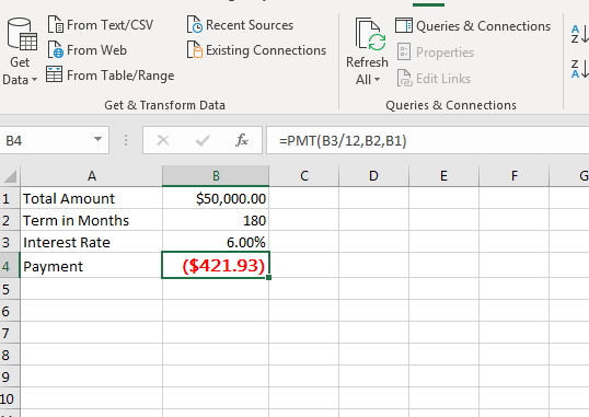
(Goal Seek data set)

The test data has 6% as a default interest rate, which displays a result. Make sure that you configure this cell as a percentage number and use ".06" as a value. In this example, a 6% interest rate on a $50,000 loan requires a payment of $421.93 for 180 months. Suppose that you want to lower the payment and need to find the right interest rate.

Select the cell that contains the PMT function. Click the "What-If Analysis" button and select "Goal Seek" from the dropdown. A window opens where you set up your values.

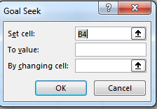
(Goal Seek setup)

Since the PMT cell was selected, the "Set cell" value is already set. The "To value" text box is where you set your desired goal. Because this is a payment goal, the value should be negative. Suppose that you want to get your payment down to $300 per month. Enter "-300" in the "To value" text box.

Click the up arrow button next to the "By changing cell" text box and select the interest rate cell B3. Click "OK" and Excel automatically calculates and shows the interest rate that you must get to pay $300 per month.

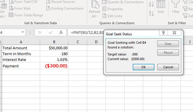
(Goal Seek result)

You can change values including the total loan amount and term in months to find the right results that match your goal. Each change will calculate to a new monthly payment that you can then use to change an interest rate value and determine your new payment. This tool will let you see results by changing a value until you're able to come up with a viable option for your budget.

Creating Data Tables

Using the payment per month example in the Goal Seek section, suppose you want to see several different interest rate options and the results of each one. A data table is beneficial when you want to see more than just one result. The data remains the same, but you can see how much you'll pay each month by factoring in several different interest rate options. To test this tool, you first need to set up your initial data.

(Data Table data setup)

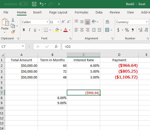
In this example, three rows are used to set up three possible payments. The term in months are 60, 72 and 48. An initial interest rate is set up to test the monthly payment for the first row. Use the same PMT function used in the previous example, but remember to change the cell references. The D2, D3 and D4 values should be the following in your data set:

=PMT(C2/12,B2,A2)

=PMT(C3/12,B3,A3)

=PMT(C4/12,B4,A4)

The C7 cell is set to point directly to the D2 cell, which calculates a payment based on 60 months and a 6% interest rate. But suppose we want to know how much a payment would be using the dame data but several different interest rates. We have 8% and 9% along with a cell that points directly to the original calculation in D2.

Selected the range shown in the image below.

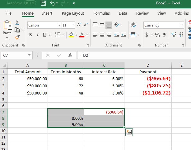
(Data Table selection)

This selection is where your Data Table is located. The cells under the original payment in C7 will show alternative payment amounts based on the other interest rates. You can set up several interest rates to see each option in the C column.

Click the "What-If Analysis" button and select Data Table. A window opens asking for input cells.

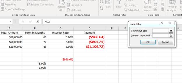
(Data Table configuration)

The column input cell should be the interest rate in C2. Since we selected the data table range and only have one input variable, click "OK." Excel 2019 calculates each option based on the interest rates entered in the Data Table.

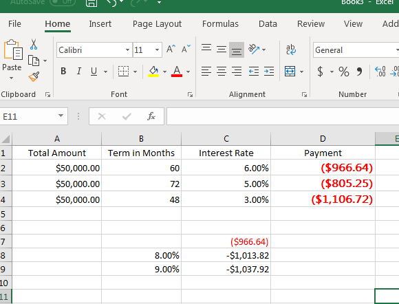
(Data Table results)

Notice that the calculation is shown under the original interest rate value of $966.64. With a Data Table, you know that if you pay 8% interest rate you'll pay $1,013.82 per month, and at 9% interest rate you'll pay $1037.92 per month.

You can make additional tables to calculate differences in other variables such as loan amount and terms in month. Data Tables are valuable when you have several different factors that can make differences in an end result.

Setting up What-If reports help with several forecast and financial calculations and possibilities. These reports can often be more complex than simple formulas and calculations, but using Excel 2019 for each scenario, data table and goal seek you'll find that it's much easier and convenient than working with expensive, advanced software on the market.