As you type content into an Excel spreadsheet, you'll notice that the software automatically formats it based on the input type. String values (alphanumeric characters) are automatically formatted with a left alignment. Numbers are automatically formatted with a right alignment. In addition to formatting the alignment for cells, Excel has several other ways to display content. You can format cells with different borders, fonts, colors and numerous other styles. This article covers the common format options that you can do with Excel.
Formatting Numbers in Excel 2019
It's common for users to work with Excel to track numerical data. Excel has a number of pre-formatted templates that you can use to display numbers a specific way. For instance, suppose that you're working with a financial spreadsheet. You want to display money values with two decimal points. If you type two zero decimal point numbers into a "General" formatted cell, Excel 2019 automatically truncates the two zeros and displays only the whole integer number.
Type the following into a cell:
15.00
Notice that Excel changes the displayed value as "15" without the two zeros and the ending decimal point. You can change this behavior by changing the format template used for the cell that stores your decimal number.
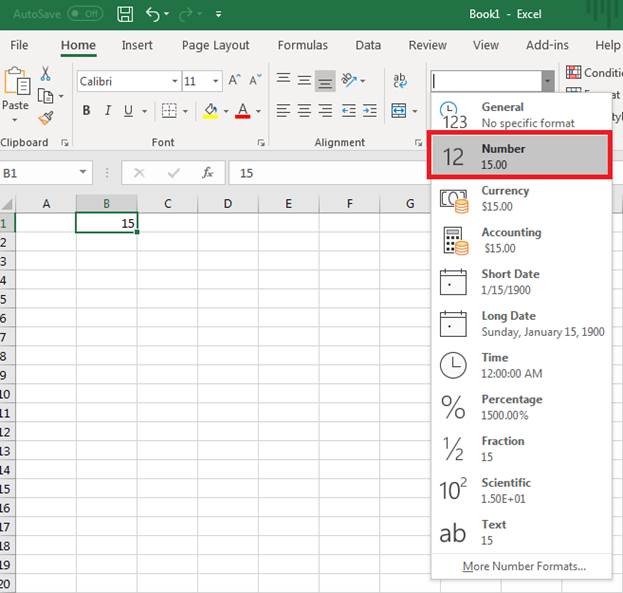
(Formatting a cell with decimal point numbers)
In the "Home" tab, click the dropdown in the "Number" section. A list of options is displayed that you can see in the image above. By default, Excel formats numbers using the "General" template. This general template detects the type of input and formats it based on Excel's detection of the value. Notice that the second option is "Number" and it displays the "15" input and what it will look like after the format is applied. In this example, two zeros were added after the decimal point, and this is the numeric format that we want. Click the "Number" option and notice that the "15" input value is changed to include the two decimal points.
Notice that the option after "Number" is "Currency." If you add a currency character to your Excel cell, you change the input from a number to a string of characters. Excel 2019 no longer detects input as a numeric value. To add special characters to a cell such as a currency character, you can use the Currency template. With the "15" input value selected, select "Currency" from the dropdown menu in the "Number" category. Notice that the cell changes from "15" to "$15.00" and is still considered numeric input.
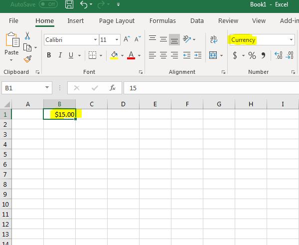
(Cell formatted with Currency)
You can test each one of the number format options from the dropdown to view results and changes in the numerical format.
You aren't stuck with just the preset number templates. You can also create your own format using the "Custom" option. Click the number format dropdown again and click
"More Number Formats" at the bottom. A new window opens with a list of options.
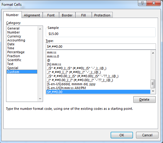
(Additional number format options)
Click "Custom" to create a custom format. Notice that several formats are shown to help you create a custom template for your cell. You'll also notice the characters used to set up the template.
For instance, look at the time format with the string "[h]:mm:ss" as the format. The "h" indicates that the first input value is the hour. The "mm" string means that two numbers must show, and these two values are the minutes. The last set of numbers is the seconds and "ss" is used to indicate these values.
Cell Styles
Some people like to separate and organize data by colorizing cells. Excel 2019 has several pre-made formats, so that you don't have to come up with an attractive layout for your spreadsheet.
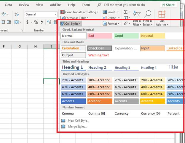
(Preset colorized styles for Excel cells)
In the image above, notice that several colors and styles are already created for you. By clicking on any one of these styles, the cell selected as all fonts, colors and background colors update to the new selection.
You aren't limited to just one cell selection either. You can highlight a group of cells and have all of them update at once. This method is beneficial when you have a header row, for example, that you want to change to a different style to have them stand out.
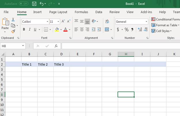
(Multiple cells in a row with changed styles)
Notice in the image above that multiple cells with "Title" text have a different background color and font. This was done by selecting all cells at once and clicking the "Cell Styles" dropdown in the "Styles" category. Select a style and all cells have the selected style applied. If you make a mistake and highlight too many cells or select the wrong style, remember that you can always click the "Undo" (arrow pointing to the left) on the top quickbar in Excel.
Font Styles
Excel has a default font that it uses with every newly created spreadsheet, but you can set your own fonts styles. The different font styles are found in the "Font" section of the "Home" tab.
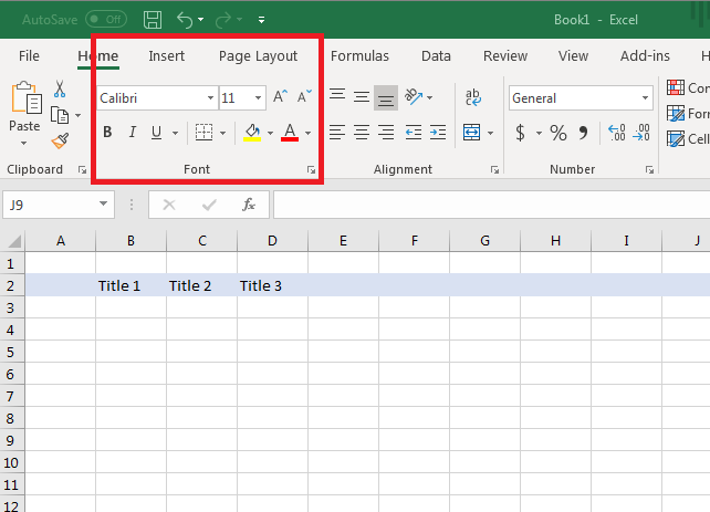
(Font style options)
If you're familiar with any type of word processors that let you create documents, you should recognize the font style options that you see in Excel 2019. The Calibri font is the default for all new Excel spreadsheets that you create. By clicking the dropdown, you see several other font options. Note that the only fonts available in the dropdown are ones installed on your computer. To add a new font, you need to download it and install the new style on your computer.
As with other styles, only the cells selected will have the new font applied to their styles. If you want to apply a style to the entire spreadsheet, you can highlight all cells in the spreadsheet using the triangle icon above the first row and the left of the "A" column.
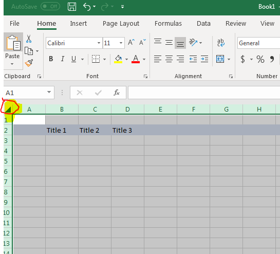
(The "select all" triangle icon)
Click the triangle icon and notice that all cells are highlighted. With these cells highlighted, choose a font or any other style and all cells have the new style applied. Click the icon again to de-select cells. This triangle icon makes it easy to quickly apply styles on all cells while still being able to apply different styles to the rest of the spreadsheet.
In the "Font" category, you see several other font style options. The "B" icon bolds font in selected cells. The "I" changes font to italicized. The "U" icon underlines text stored in a cell. Click all three of these buttons to apply underline, bold and italicize styles to cells.
The dropdown next to the font dropdown is the size option. By default, Excel sets the size of your cell's text at 11. This font size can be increased or decreased by selecting the appropriate size from the dropdown. You can also change the size of the font by clicking the "A" buttons next to the font size option. The "A" button with an up arrow increases the size, and the "A" button with a down arrow decreases the size.
The final important two buttons are the paint bucket icon and the "A" icon with an underline. By default, the underline is red, which means that by selecting a cell and clicking this button you change the font color to red. Click the "A" with the underline button and you'll see a list of color options. Notice at the bottom of the color list is "More colors." Click this option and a window opens where you can customize a color or pick a shade of a specific color. Excel lets you enter a hexadecimal value for a color, which provides you with every color that you can think of for your fonts.
The paint bucket sets the background color for a cell. It works similarly to the font color dropdown. Click the button and a list of colors are displayed. It also has the "More colors" option where you can choose a custom color or a shade of an existing one. Clicking a color changes the background of all selected cells.
Text Alignment
There will be times that you want to set different text alignment with multiple cells. Excel 2019 has an "Alignment" section in the "Home" tab with several alignment options.
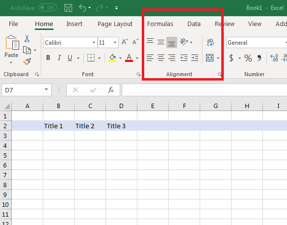
(Alignment options for Excel cells)
Alignment within cells can be made both vertically and horizontally. The first row of alignment icons set the alignment vertically. Vertical alignment options are top, middle and bottom of the cell. The second row of buttons sets the horizontal alignment. The first one aligns text to the left (which is the default for Excel), the second centers text, and the third one sets the alignment to the right.
The button to the right of the alignment buttons is the "Merge" function. By merging cells, you combine the number of cells selected into one. Excel treats merged cell as the same cell even though these cells take up multiple rows or columns.
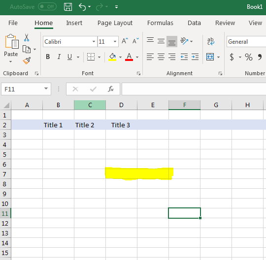
(Two merged cells)
In between the horizontal alignment buttons and the merge button, you see alignment icons with arrows pointing to the left and right. These buttons increase or decrease the indent. When you have large blocks of text, you might want to use an indent for some of the text. By clicking the button with the left arrow, you decrease the indent. Clicking the button with the right arrow increases the indent to the right.
Two more buttons above the indent options work with the way text displays. The first one lets you arrange the way text displays. For instance, change text from displaying horizontally to vertically. The second icon wraps text if it's longer than the width of a column. Excel automatically increases the size of a row when words wrap to a second line within a cell.
Formatting cells is the way you make attractive spreadsheets either for yourself or a business. With Excel's numerous quick buttons, you can change colors, font, alignment and size of your text within a few seconds.