Setting Up Data

When you sort and conditionally format data, usually it's a large number of rows. The following examples use a set of data with 20 rows. The data represents a list of customers and the amount of revenue made from each sale.

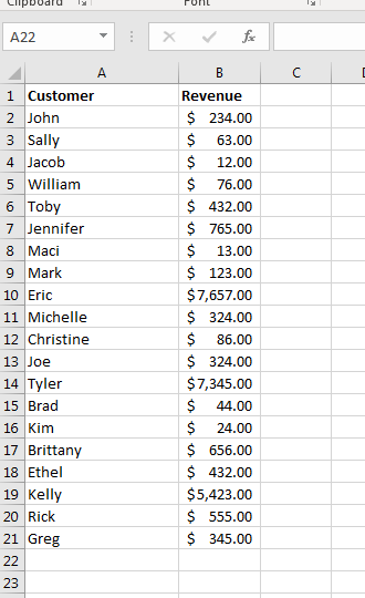
(Data setup for sorting and formatting examples)

Notice that headers are used at the top of each column. This is important for sorting when you want to change the column to sort on. Excel's sorting functionality is handy even when you only have a few rows. If you want to view a list of revenue numbers based on the highest value or lowest value, instead of eyeing values and determining the right one based on your own human review, Excel 2019 will ensure that you can sort values and find the ones that have the highest revenue.

Sorting Data

Excel offers a few options for sorting data. First, you can sort one column of data with only a click of a button. To set an order on just one column, selected the column by clicking the letter label at the top. With the column selected, Excel gives you two buttons to either sort by ascending or descending values.

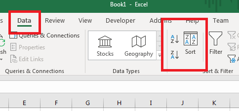
(Excel sort buttons)

The two buttons to the left of the "Sort" button shown in the image above. You can also sort a selected range of cells and order only selected data. Copy and paste a small section of the test data to a separate column. Highlight only these cells and then click the sort order that you want to set for the selected range. The button that shows an arrow pointing down with the first letting being A will sort values in ascending order. The button that displays an arrow pointing down but the first letter is Z will sort values in descending order.

Excel can identify if your data is a set of dates, textual values or numbers. The sort function then orders cells based on the detect data type. For instance, if you have a list of revenue sales, Excel knows to sort cells based on numeric values. If you have cells formatted as dates, Excel knows that these values should be ordered in chronological order. Cells that are text values such as customer names are ordered alphabetically.

Since we have a spreadsheet of customers and their revenue, we have two columns to sort. If you use the single-column sort buttons, Excel only orders one column, and your data is corrupted. The "Sort" button takes care of this issue by providing a way to keep your columns connected but sort data based on the column that you want to use for the sort.

The first step is to highlight the cells in our spreadsheet. Make sure you include the column headers, because Excel uses them as part of the sort function. Click the "Sort" button and a window opens asking for input.

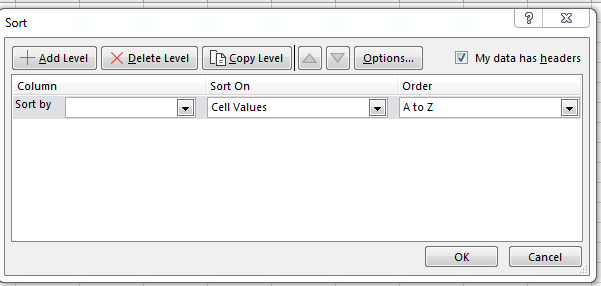
(Sort configuration window)

The "Sort By" dropdown has the headers for each column listed. Since we have "Customer" and "Revenue" as a column header, these two values display in the "Sort By" dropdown. If you don't have column headers, Excel lists the column letter labels. Should you have several columns, having only letter labels make it difficult to configure your sort order.

The "Sort On" dropdown defaults to "Cell Values," which means that the value is used for the sort. This is the typical configurations, but you can also sort on cell color or font color. This is useful when you set conditional formatting, which is covered in the next section.

The "Order" dropdown indicates if you want to sort data in ascending or descending order. The "A to Z" option means that you want to sort data in ascending order. The "Z to A" option means that you want to sort data in descending order.

In this example, let's sort on the "Revenue" column and leave the other dropdown options set to the default. Click "OK" to sort your data.

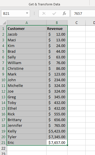
(Data sorted by "Revenue")

Notice that names still match up with revenue values. This is because the "Sort" functionality knows to keep rows aligned even though you're ordering data by one column. If you decide to change the order to customer names, repeat these steps and choose "Customer" from the "Sort By" dropdown. Columns are still aligned properly but rows are ordered again based on the customer's name.

Conditional Formatting

Sorting data doesn't highlight certain cells that might need to stand out among the others. For instance, you might want to know which customers had revenue within a specified range. You might want to know which customers had revenue under or over a certain threshold. You can sift through all of your records, but conditional formatting that changes the font or background makes these cells stand out much more and makes them easier to find. With a short customer revenue list that contains only 20 rows, you can easily find the customers that bought and added revenue to your income, but if you had thousands of records even a sorted list would make it difficult to find specific records.

Excel has a function called "conditional formatting" that changes the color of a cell's font or the background color of a cell to make it stand out and easy to find when you're looking for certain values that meet a condition.

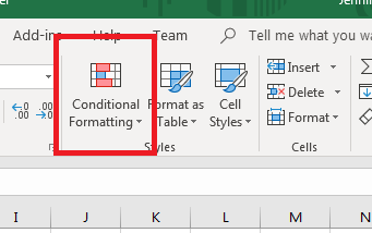
(Conditional Formatting button)

The "Conditional Formatting" button is found in the "Home" ribbon tab. The image above shows the Conditional Formatting button, which is also in the "Styles" category.

Select only the currency cells before you set conditional formatting. If you highlight all of the cells including customer names, Excel 2019 won't be able to differentiate text from currency values and won't highlight the right cells. When you click the button, several options are shown in a dropdown list.

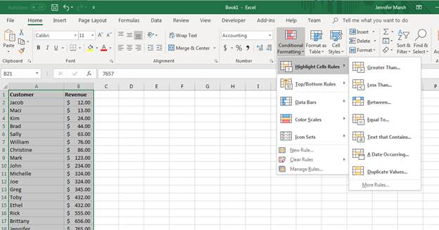
(Conditional formatting dropdown options)

As you can see from the image above, conditional formatting gives you several options. The most common function used is "Highlight Cell Rules," which if you click also has several options. These options are perfect for numeric values when you want certain cells to stand out among the rest. You can choose greater than, less than, between and equal to. These options let you find revenue for customers based on the amount of money they brought in according to the spreadsheet.

With conditional formatting, you aren't limited to just one color with one condition. You can set multiple colors using multiple conditions. For instance, you might want to know which customers brought in revenue under $100 and which customers brought in over $1000. You can then take this data and use it for reporting and product information. Using revenue charts and conditional formatting, you then know which customers are the best (or worst) to market to and upsell additional product.

In this example, we want to know which customers brought in revenue over $1000. Again, you can eye this information by just looking at the twenty records with rows sorted in descending order using the sort function. But think of a spreadsheet with thousands of records and how difficult it would be to find all customers even if those rows are sorted in ascending or descending order.

From the "Highlight Cells Rules" dropdown options, choose the "Greater Than" option. This opens a new configuration window.

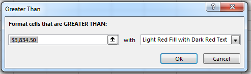
(Greater than conditional formatting configuration window)

Notice that a value is automatically filled in. This default value gives you a mid point to set your conditional formatting, but you will likely need to change this setting to a value of your own. We want to know which values are greater than $1000, so enter 1000 in the value input text box. If you click the up arrow, you can also select a cell to be your configuration value.

As you change the value in the input text box, Excel 2019 shows the cells that will change in your selected group of cells should you click the "OK" button. If you pressed the up arrow button, press "Enter" after you are done selected a value or type a value into the input text box and press "Enter."

The next dropdown lists the colors for both the background of a cell and the font. The default is a light red (pink) fill with a darker red font color. You can also choose to only have the background color changed or change only the font color. Click the dropdown to see a list of options and colors. In this example, we'll use the default option and change the color of both the cell's background and the font foreground.

Click the "OK" button to see the results in your spreadsheet.

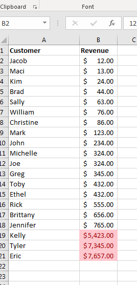
(Conditional formatting set on cells greater than $1000)

With conditional formatting, you can now quickly see which customers brought in revenue over $1000. This formatting persists even when you sort cells again using the "Sort" option. Should you decide to use other conditions, you can make them other colors to make it easy to distinguish between the two conditions.

One reason many businesses use Excel 2019 is because of the many options available when charting and sorting data. Sorting data makes it much easier to make a quick review of your data, and you can also make it easier for other users to find information easily when they are unfamiliar with the data. Conditional formatting provides an added aesthetic touch especially when you have thousands of records that must be reviewed. Conditional formatting can actually save hours in charting and review time for anyone that needs to look at numbers in an Excel 2019 spreadsheet.

Once you understand the way conditional formatting and sorting works, you can make it much easier to work with large data sets that must be evaluated each month, especially revenue sheets.