Formatting a worksheet can change the look and feel of it. You can add color, change fonts, put in things such as headings, apply styles, and much more. Taking the time to format a worksheet can take it from the black and white page of data and gridlines to something that looks professional and attractive.
Change Font Size and Type
Font is defined as the style of your type. Times New Roman, Courier, and Arial are probably three of the most popular fonts, but there are literally hundreds. When you create a worksheet, you can decide what type of font you want to use. You can also decide the size of the font.
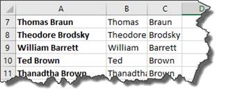
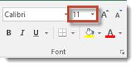
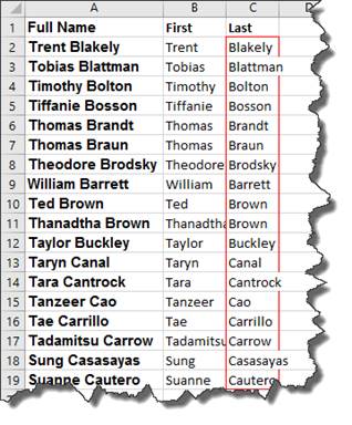
In the snapshot below, we've used Calibri, size 11 font.
However, we can change that to another font and another size.
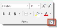
To change the font type and size, go to Font group under the Home tab.
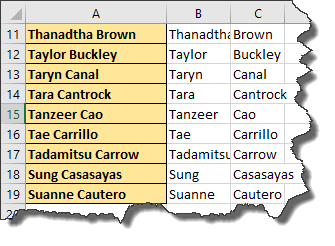
Next, select the data in the worksheet for which you want to change the font. We've selected column A in the snapshot below.
Go to the Font group, and you'll see the type of font that you're currently using. It appears in a box with a downward arrow beside it on the left hand side of the toolbar. In our example, and on our toolbar, it's Calibri.
Click on the downward arrow to the right font type and select a new font.
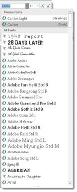
We're going to select Arial.
Once you select the font, the selected data will be changed to the new font.
To change the size, select the cells, then click the downward arrow beside the current size.
Font Attributes
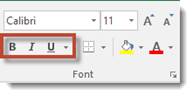
You may want to select boldface, italicize, or underline data inside cells. The boldface command in MS Excel is represented by an uppercase, boldfaced B. Italics are represented by an uppercase, italicized 'I', and underline by an uppercase U with a line under it. These buttons are located directly below the font type window in the Font group.
To add italics, boldfaced, or underlining to data in cells, select the desired cells, then click the appropriate button (B for boldfaced, I for italic, or U for underline).
By clicking the downward arrow to the right of the underline button, you can choose an underline style.
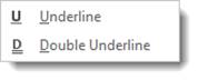
You can choose the standard underline, which is a single line. You can also choose the double underline, which is two lines.
Add Borders to Cells
You can also add borders to cells or a range of cells by selecting the cell(s) you want to add border to, then by clicking Border button in the Font group under the Home tab.
It looks like this:

When you click on the Border button, you will see this dropdown menu:
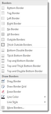
Simply select where you want to border to appear and what kind of border you want. Keep in mind that the border you choose will be applied to a single selected cell or to a range of selected cells.
You can also change the line color of the border and the border style (such as dashed or solid lines) by going to the Draw Borders section of the dropdown menu.
Let's see how it works.
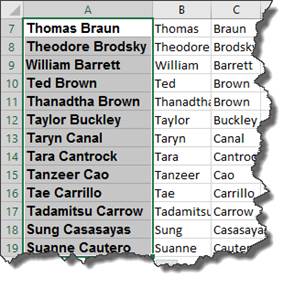
We want to apply borders to the cells in column A.
As you can see below, we've selected the cells.
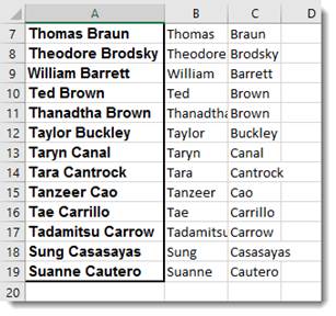
Next, we go to the Ribbon and click the Borders button.
We choose Thick Outside Borders.
Since we selected a range of cells, the border is applied to the entire range, not the individual cells.
Let's do something a little different now. Instead of applying a border, we're going to go to the Draw Borders section of the dropdown menu. We're going to draw borders.
Select Draw Border from the dropdown menu.
When you draw a border, your mouse cursor turns into a pencil. You can click the border of a cell to add a border. You can also drag your mouse over cells to add a border. We are going to drag our mouse over column C.
You can also choose to add a line color or a line style for the border you draw. We're going to choose Line Color from the dropdown menu, and choose the color red. Once again, you can click the border of a cell to add a border. You can also drag your mouse over cells to add a border.
Font Color
Changing the font color is as easy to do as changing the font. By default, your text in Excel 2016 appears in a black font. If you want to change the font color, look for the uppercase A with a colored bar under it in the Font group under the Home tab.
Select the cells for which you want to change the font color, then click on the button to choose the color you want to apply to the selected text.
Add Color to a Cell or Range of Cells
You can also add color to a cell or range of cells. This doesn't change the font color, but instead provides a colored background.
To the left of the font color button, you'll see what looks like a paint bucket with a yellow bar underneath it. Simply select the cells you want to give a color, click the button, and select the color of highlight that you want to apply.
In the example below, we chose a yellow.
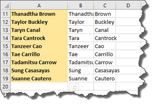
Please note that the cell borders that show up in Excel by default are no longer displayed when we add color. If you want borders, you have to add them.
We selected All Borders from the Borders dropdown menu, then dragged over the cells in column A to apply the borders.
The Format Cells Dialogue Box
Click the arrow in the right side bottom corner of the Font group to access the Format Cells dialogue box.
The dialogue box looks like this:
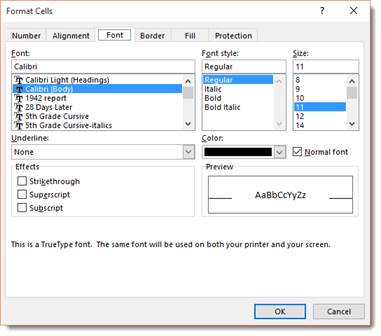
From this dialogue box, you can format your data just as you did from the Ribbon. The Preview section of the dialogue box lets you preview your changes before you apply them.
Click OK when you're finished making changes to apply them to your spreadsheet.
Formatting with the Mini-Bar
The mini-bar appears whenever you right click within a cell.
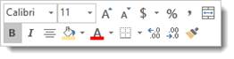
In the snapshot above, you can see that it contains the tools to change the font, font size, etc. You can use this to format your cells to save the time you'd spend going to the Ribbon.
Merge Cells
Merging cells simply means that you merge a group of cells into one cell. It is not the same as combining cells because when you combine cells, the data in those cells is also combined.
When you merge cells, the information in the upper left cell is centered in the merged cell. If the content you want in the merged cells is not in the upper left cell, then you must copy and paste the data into the upper left cell.
Note: It's important to remember that the cells you merge must be adjacent. In addition, the cells that you merge cannot be active or the Merge and Center feature will not work.
To merge cells, first select the cells to be merged.
Go to the Alignment group under the Home tab, then click Merge and Center.
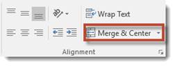
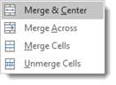
Select an option from the dropdown menu.
Apply Number Formats and Create Custom Number Formats
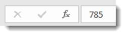
You can change the appearance of numbers in MS Excel 2016 without changing the value behind those numbers. The actual value is always displayed in the Formula Bar.
For example, we can have a numbers formatted as currency in the worksheet:
Yet, if we click on a cell in the Formula Bar, the number is displayed as a general number.
You can apply a number format to a cell by selecting the cell(s) that you want to format, right clicking, and selecting Format Cells and select the Number tab.
You can also to the Home tab, go to the Number group, then click on the arrow in the bottom right corner.
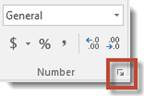
You will then see the Format Cells dialogue box. Click on the Number tab.
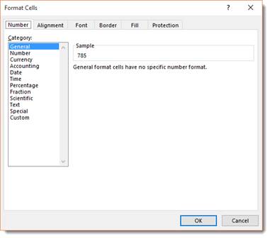
In the dialogue box above, you can choose the type of number formatting that you want from the Category column. An explanation of how the formatting is used appears at the bottom of the dialogue box when you click on a specific type of number formatting.
We chose Currency from the Category column.
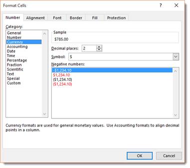
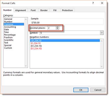
We wanted two numbers to appear after the decimal point.
We wanted to use the American dollar symbol.
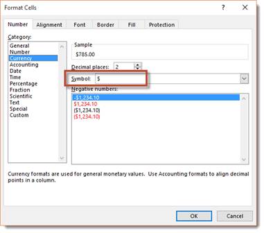
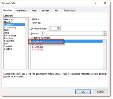
We wanted negative numbers to appear with the minus (-) sign before them. We could have also chosen to have them appear in red, black with parentheses, or red with parentheses.
Click Ok when you're finished.
Creating Custom Number Formatting
If the number formats the Excel provides won't work for your data, you can create a custom number format. To do this, go to the Format Cells dialogue box again, and click Custom n the category column.
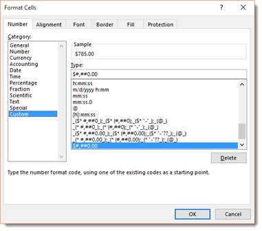
In the Type list, select the format that you want to customize. As you can see in the snapshot above, we chose the currency format.
Now go to the Type field and customize the format by entering the format you want to use.
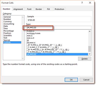
Click OK when you're finished.
Align Cell Contents
You can align the data in a cell to the left, right, or center.
To align data to the left means to align it to the left side of the cell. Simply select the cell(s) that contain the data that you want to align to the left.
Go to the Alignment group under the Home tab.
Click:
 To align to the left.
 To align to the right.
 To align to the center.
 To align data to the top of a cell.
 to align data to the middle of the cell.
 To align data to the bottom of the cell.
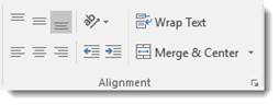
About Indents
You can also indent data in cells. When you increase indent, you increase the margin between data in the cell and the left cell border.
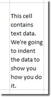
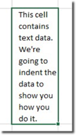
The cell pictured below has text data in it.
Select the cells that contain data that you want to indent. Then, go to the Alignment group under the Home tab.
The two buttons highlighted below allow you to decrease indent (first button), or increase indent.
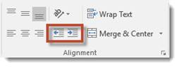
We're going to increase the indent (second button).
About Text Wraps
Text wrap will wrap the entries from selected cells that have data that spills over their right borders.
Here's an example:

Select the cell(s) you want to apply text wrap to, then click the Wrap Text button in the Alignment group under the Home tab.

The text is then wrapped within the cell.
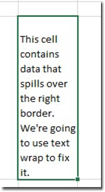
As you can see, the text is now wrapped to fit between the left and right borders of the cell.
Changing the Orientation of Cell Entries
Instead of wrapping text in cells, you can also change the orientation of the text by rotating the text up or down. This can work well with labels in worksheets.
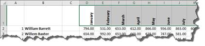
In the example below, we're going to change the orientation of the data that contains the days of the week.
To start with, we've selected the cells that contain this data:

Next, we go to the Alignment group under the Home tab and click the Orientation button. It looks like this:

From the Orientation dropdown menu, we now we get to choose the new orientation:
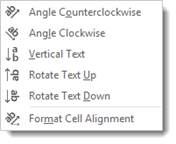
We're going to choose Rotate Text Up.
You can see that our column labels are now vertical with the text going upward (from bottom to top).
The Format as Table Gallery
The Format as Table Gallery is a way to format your cells without having to select the cells first. Think of it as a shortcut to formatting cells. Your cell cursor just has to be within the table of data right before you click the Format as Table button that's located in the Styles group under the Home tab (pictured below).
We're going to put our mouse cursor in a cell by clicking on the cell.
Now we're going to go to the Format as Table button and look at the gallery.
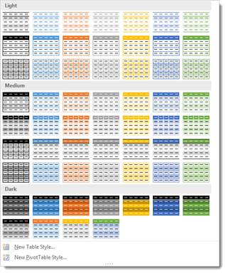
Choose a formatting style that you want.
When you click on a style that you want, you'll see the Format as Table dialogue box.
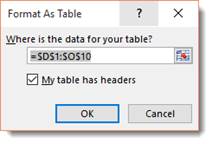
This contains the cells referenced for the formatting. In the dialogue box pictured above, Excel has the referenced cells listed as D1 through O10. If this is incorrect, you can change it.
Put a checkmark beside "My table has headers" if your data has headers. Ours does. The headers are the column labels. In our example, the headers are the months of the year.
Click OK when you're finished.
The Table Tools Design tab then opens in the Ribbon.

Located under the Table Tools Design tab is a Table Styles Options group that allow you customize your table even further.
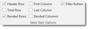
Header Row adds formatting and filter buttons to each of the headings in the first row. Ours already has filter buttons (the down arrow)
-
Total Row goes at the bottom of the table for totals.
-
Banded Rows means shading will be applied to every other row.
-
First Column puts row headings in the first column in boldface.
-
Last Column puts row headings in the last column of the table in boldface.
-
Banded Columns applies shading to every other column.
In the Table Styles group, you can also change the style of table that you applied when you chose a format for your table from the gallery.
Our table now looks like this:
Conditional Formatting
Conditional formatting is a neat little feature of Excel 2016 because it helps you do your job better. Let's say that you're entering in sales figures for each employee into a spreadsheet. Your boss has told you to let him know if anyone sells less than $300.00 worth of products in a given month. Did you know that you Excel can notify you each time this happens? You can program Excel 2016 to give you a "red flag" every time a certain situation exists.
To apply conditional formatting, go to the Styles group under the Home tab. Click the Conditional Formatting button. You will see a dropdown menu.
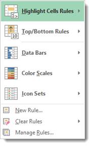
Let's learn what each of the options does for you:
-
Highlight Cells Rules allows you to define rules that highlight the cells in the cell selection when certain values such as text or dates that have greater or less than a value that you specify or fall within a range of values.
-
Top/Bottom Rules gives you options for defining rules that highlight the top and bottom values, percentages, and above and below average values in a cell selection.
-
Data Bars opens a palette with different colors of data bars. You can apply these to a cell selection to indicate their values relative to each other.
-
Color Scales opens a palette with different color scales that you can apply to a cell selection to indicate their values relative to each other.
-
Icon Sets will open a palette with icons. You can apply these icons to a cell selection to indicate values relative to each other by clicking the color scale thumbnail.
-
New Rule allows you to create new rules.
-
Clear Rules allows you to remove conditional formatting rules for the cell selection.
-
Manage Rules opens a dialogue box where you can edit and delete rules.
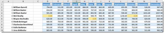
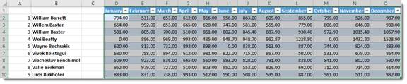
Let's apply conditional formatting to our spreadsheet.
We're going to use Highlight Cell Rules.
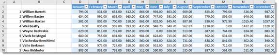
First, we select the cells. This is our cell selection.
Now, we go to the Conditional Formatting button on the Ribbon and choose Highlight Cell Rules.
We want to cells to be highlighted when a value is less than 300. We chose Less Than from the side menu that appears when you click Highlight Cell Rules.
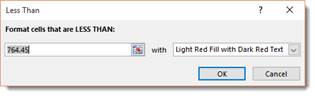
We want to format cells that are less than 300, so we're going to enter that into the box.
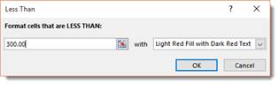
Next, we choose what colors we want to use to highlight the cells that have values less than $300.
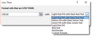
We are going to choose Yellow Fill with Dark Red Text.
Click OK when you're finished.
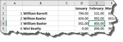
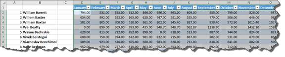
As you can see in our snapshot below, the cells less than 300.00 are now highlighted.
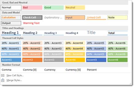
Creating and Applying Styles
If you frequently use the same formatting options for the cells in your worksheets, you may want to create a formatting style to save you time. A formatting style is a collection of formatting choices. It may include-- but not be limited to-- font, font size, and color.
To create a new style, first format a cell with the selection of styles that you want.
Select the cell.
We've selected the cell below as our example:
Next, go to the Home tab to the Styles group, and click the downward arrow to the right of the Styles gallery.
Select New Cell Style from the dropdown menu.
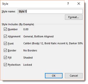
Create a name for the style in the Style Name field, then choose the formatting options that you want to include in the style.
Click OK when you're finished.
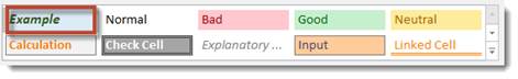
As you can see, our new style now appears as the first style on the left in the Style Gallery.
NOTE: You can also apply pre-created styles from the Style Gallery and apply them to cells or ranges of cells. To apply a style, select a cell or range of cells, then choose the style from the gallery that you want to apply.
Formatting Using Quick Analysis
Quick Analysis is a feature that was new to Excel 2013. It can make doing things such as creating charts, adding sums, or even formatting cells easier than ever before. In fact, you can do it in as little as two clicks of the mouse.
To format cells using Quick Analysis, first select the cells that you want to format.
When you select your cells, you'll see the Quick Analysis button appear at the bottom right of the selection. We highlighted it in red below.
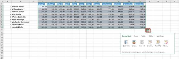
Click on it and the Quick Analysis tool opens. We have now highlighted it in red.
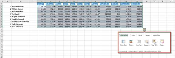
Let's zoom in and get a better look at it:
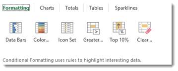
By default, Formatting options are shown to you when you click on the tool. From here, you can apply conditional formatting the same way as we learned to do earlier in this lesson. You can also work with charts, totals, tables, and sparklines.
The Format Painter
The Format Painter tool is located under the Home tab in the Clipboard group.
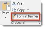
The Format Painter looks like a broom, but it acts more like a paintbrush.
Using it, you can "borrow" the formatting from cells or selections of cells and apply the same formatting somewhere else. It's operates a lot like the "copy" function in Excel, except instead of copying text, you're copying formatting.
To use the Format Painter, select the cell or cells for which you want to copy formatting.
Now, click the Format Painter button. You'll notice that the cursor changes to a paintbrush.
Next, select the cell(s) you want to change to paint with the borrowed format.