It would be a big mistake for anyone to chalk Excel up to a fancy calculator that simply creates fancy spreadsheets and performs calculations. It's much more than that. It can also perform what-if analysis.
There are all types of what-if analyses that Excel can do. However, in this article, we're going to cover three:
-
Data tables. This lets you see how changing one or two values will affect the bottom line.
-
Goal seeking. This lets you to discover what it takes to reach a certain objective.
-
Scenarios. This lets you set up and test different cases (best case scenario).
Data Tables
Excel 2016 will support two types of data tables: a one variable data table and a two variable data table. The one variable data table substitutes a series of possible values for a single value in a formula. A two variable table substitutes a series of possible values for two values in one formula.
If you're lost as to what we mean at this point, don't worry. Let's walk through it step by step. We're going to do a what-if analysis with a one variable data table.
To start a what-if analysis, click the Data tab, then go to the What-if Analysis button in the Forecast group.
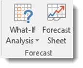
Choose Data Table from the dropdown menu.
You'll then see this dialogue box:
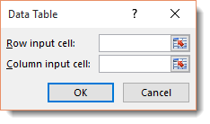
The dialogue box above has two text boxes: Row Input Cell and Column Input Cell.
If you're creating a one variable data table, you choose one cell in your worksheet to use as either the Row Input Cell or as the Column Input Cell.
If you're creating a two variable data table, then you fill in both text boxes. One cell becomes the Row Input cell that substitutes values you've entered across columns of a single row � and vice versa.
Let's create a one variable data table to start with.
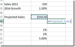
The spreadsheet shows sales forecast for a convenience store.
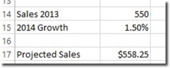
In cell B17, pictured above, we've calculated our projected sales by adding last year's sales and the amount we expect it to grow.
Here is the formula we used.
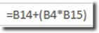
Because we went to the Formula tab and clicked Create from Selection, then chose Left Column (pictured below), our formula reads:=Sales-2016+(Sales_2016*Growth_2014).
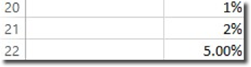
Now, note that we've entered various growth rates in cells B20 through B22 . We're going to insert these various values into the growth formula.
Here's how we do it.
Copy the formula from B17 into C18 by going to cell C18 and typing the equal sign, then clicking on cell B17. By doing that, you've created the formula =Projected_Sales_2014.
Hit Enter.
Next, select the cell range B20:C22.
Go to the Data tab and click What-If Analysis, then Data Table.
Click on cell B15 in the Column Input Cell, then click OK.
The projected values are then listed.
Now click cell C18, then click the Format Painter. Drag it through cell range C20-C22.
Goal Seeking
Use Goal Seek when you already have an outcome in mind, such as a target sales amount. Goal Seek will allow you to figure out the numbers you need to hit to reach your goal.
To use Goal Seek, you click the What-If Analysis button and select Goal Seek from the dropdown menu. You'll need to select the cell that contains the formula with the result you want. This is called the Set Cell. Next, you'll indicate the target value that you want the formula to return, in addition to the location of the input value that can be changed to reach this target.
Let's show you what we mean.
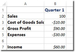
In the table above, we want to figure out how much sales will have to increase to reach a first quarter income of $100.
We'll start out by selecting cell B7. Now go to the Data tab, click the What-If Analysis button, then Goal Seek.
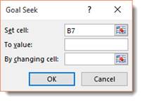
Set the To Value box to 100 because that's our goal. In the By Changing Cell field, click cell B2 (first quarter sales). Enter the absolute address.
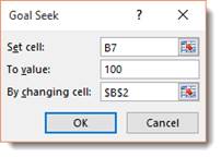
Click OK.
Now we can look at our spreadsheet.
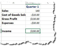
We see how our numbers must change to meet the goal.
Scenario Manager
The Scenario Manager allows you to create and save different input values that create different results. These are called scenarios.
To set up a scenario, the first thing you have to do is identify the various cells whose values can vary in the scenarios. Next, you select these cells, then click the Data tab and go to What-If Analysis, then Scenario Manager.
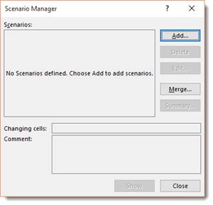
Click Add.
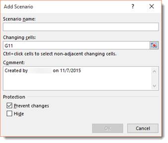
For our scenario, we're going to do Most Likely Case.
Enter Most Likely Case in the Scenario Name box.
Click OK.
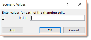
Now enter the values for the most likely case.
Click Add to add another scenario.
When you're finished adding scenarios, click OK.
Click on the scenario, then click Show to see the numbers change.
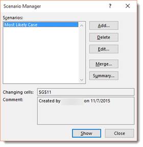
From this window, you can also produce a summary report. This shows the changing and resulting values for your scenarios, in addition to the current values.