Learning how to navigate around Excel is critical to being able to successfully use the program.
If you have access to Excel 2016, you should open a blank spreadsheet at this time.
Understanding the Basic Elements of an Excel Spreadsheet
Before going any further, it's important to understand the elements of a spreadsheet in Excel or any spreadsheet that you may use.
A spreadsheet is made up of individual cells. One cell is simply a block on your screen. In the snapshot below, you can see a cell that's highlighted:
The cell above is highlighted because it's an active cell. To make the cell active, we clicked on it with our mouse. A cell must be active in order to enter data.
All the cells within a worksheet are organized into columns and rows. In Excel, rows are represented by numbers. Columns are represented by letters. Rows go across the spreadsheet horizontally. Columns go down the spreadsheet vertically.
Since rows and columns are labeled with numbers and letters respectively, it's easy to locate the exact coordinates of a cell.
For example, instead of your boss coming to you and telling you the number for March's expenses are wrong, he can simply say, recheck the number in D15. This would tell you to go to column D, row 15.
It gets even easier. Instead of scrolling through your worksheet to find D15, simply go to the Name box above Column A. We've highlighted the name box below.
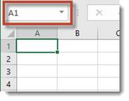
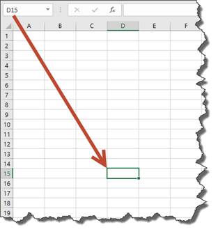
Enter the coordinates for the cell. We're going to enter D15, then hit Enter.
As you can see below, Excel took us to the exact cell and highlighted it for us.
The Formula Bar
The formula bar is the magical ingredient of the soup, so to speak. The formula bar does the math for you. For example, you can enter a formula for cell D15 into the formula bar. Excel will calculate it for you, then display the answer in the cell.
The formulas and equations that you enter will be entered in and displayed in the Formula Bar. It is located to the right of the Name Box. We have highlighted it for you below.
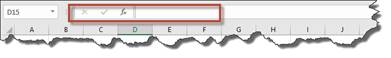
The Formula Bar has the fx to the left of it.
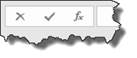
On the left side of the Formula Bar are the Formula Bar buttons. The Insert Function button is fx. When you start making or editing a cell entry, X is Cancel and the checkmark is Enter.
The white area (or bar) to the right of the buttons is the Cell Contents area.
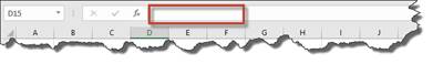
The Formula Bar always shows you the contents of a cell, even if it doesn't appear in the cell. In other words, it shows equations in the cell even if the cell only displays the answer to the equation. It will show contents of cells that appear to be blank in the spreadsheet as well. If the Cell Contents area is blank, you know the cell is empty.
The Backstage Area
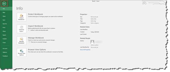
The Backstage area is located under the green File tab at the upper left hand corner of the Excel window. If you click on it, this is what you see:
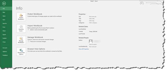
Using the Backstage area, you can open an existing spreadsheet, create a new spreadsheet, save workbooks and spreadsheets, share workbooks and spreadsheets, print, close, and set options for the Excel program.
Click the left facing arrow at the top left of the Backstage area to go back to your spreadsheet.
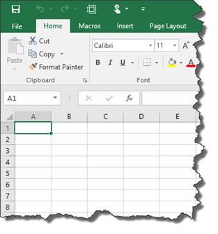
The Quick Access Toolbar
The Quick Access Toolbar is located at the top left of the Excel window. It looks like this:
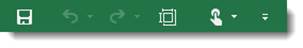
You can use the Quick Access toolbar to add shortcuts to tools that you use frequently. This is a time-saver over having to click tabs and find the tools in a group.
By default, our Quick Access toolbar displays these shortcuts:
 Save
Save
 Undo
Undo
 Redo
Redo
 Print Preview/Print
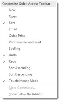
You can customize the Quick Access toolbar and add shortcuts so the tools you need appear there for easy access.
Click the dropdown menu to the right of the toolbar. It looks like this: 
Click on the shortcuts you want to add to the toolbar from the list. When you click on a shortcut, it will put a checkmark beside it, letting you know it appears on the Quick Access toolbar.
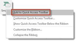
If you want to add a shortcut for a tool, but you don't see it on the Customize Quick Access Toolbar list, you can still add it to your toolbar. You do this by adding Ribbon commands. Let's show you how to do it.
1. Go to the Ribbon and find the tool that you want to add. Right click on the tool (or tab and hold if you're using a touchscreen device).
In this example, we're going to add SmartArt under the Insert tab by right clicking on the SmartArt button.
2. Select Add to Quick Access Toolbar.
If you want to move a command button in the toolbar to a different location or group it with other buttons on the toolbar, click the dropdown menu on the right side of the Quick Access Toolbar. Select More Commands.
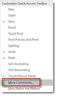
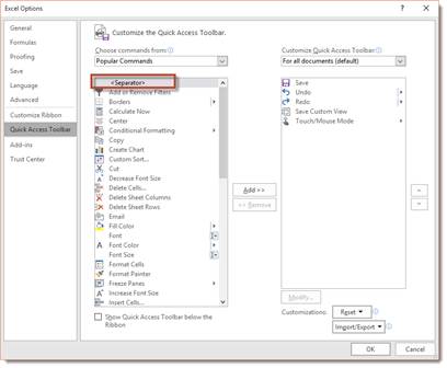
You will then see this dialogue box:
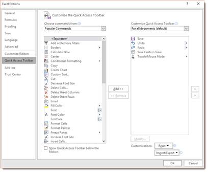
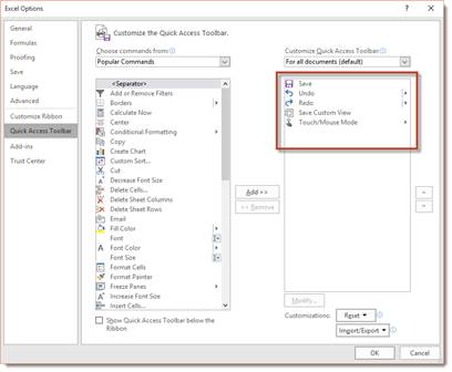
In the right column, you can see everything that already appears on the Quick Access toolbar in the order that they appear.
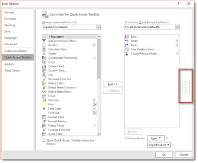
If you want to reorder the tools, click on a tool, then use the arrows to move it up or down.
If you want to group buttons together on the Quick Access toolbar, you can add vertical separators. To do this, select the tool for which you want to appear above the separator.
Now, click <Separator> from the list on the left.
Click the Add button.
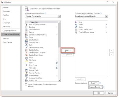
In addition to a separator, you can add any of the tools that appear in the column on the left to the Quick Access Toolbar. Simply click on the tool to select it, then click the Add button.
To remove shortcuts from the Quick Access toolbar, select the shortcut in the right column, then click the Remove button.
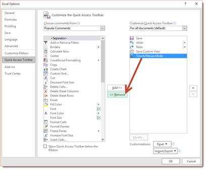
Click the OK button when you are finished.
Moving Around Worksheets
Being able to navigate through a worksheet will make using Excel a lot easier. However, before we discuss that, let's quickly review three things you have to know about the worksheet area. Remember, the worksheet area contains cells, rows, and columns.
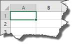
1. The cell cursor is the dark green border that appears around a cell. It means a cell is active.
2. The location of the cell, or address, appears in the Name box.
3. he active cell's row number and column letter are shaded. Look at the snapshot below. Note that the row number 1 is shaded differently than the rows after. Note that the column A is shaded differently than the other columns.
Now, since the Excel worksheet contains so many cells, rows, and columns, not all of your cells are going to be displayed at once on the screen. For that reason, there are several ways that you can use your mouse cursor to move through and navigate your worksheet.
Of course, if the cell is displayed, you can simply click on it to make it active. If you're using a touchscreen, just tap it.
You can also type the coordinates in the Name box and be taken to the cell, or you can press F5 to open the Go To dialogue box.
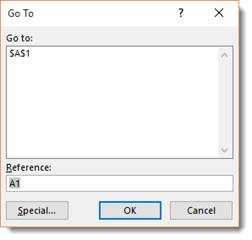
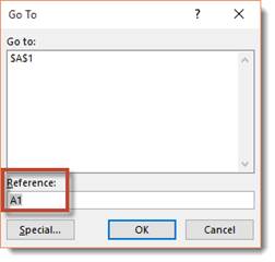
Type the coordinates of the cell in the Reference field.
You can also navigate through a worksheet by using cursor keys on yourkeyboard. The cursor keys are displayed in the table below:
|
Keystroke |
Action |
|
� On the keyboard Or Tab |
Moves cell to the right |
|
� on the keyboard or Shift+Tab |
Moves cell to the left |
|
Up arrow on the keyboard |
Moves one cell up |
|
Down arrow on the keyboard |
Moves one cell down |
|
Home |
Moves cursor to cell in Column A of the current row |
|
Ctrl+Home |
Moves cursor to the first cell- A1 |
|
Ctrl+End or End, Home |
Moves the cursor to the cell that's at the intersection of the last column with data and the last row that has data in it |
|
Page Up |
Moves the cursor to cell that's one full screen up in the same column |
|
Page down |
One full screen down (in the same column) |
|
Ctrl+� or End, � |
Moves the cursor to the first occupied cell that's to the right that's has a blank cell before it or after it. If there isn't an occupied cell, it goes to the end of the row |
|
Ctrl+� or End, � |
Same as above, except first occupied cell to the left. |
|
Ctrl+ Up arrow, or End, Up Arrow |
Moves the cursor to the first occupied column above that has a blank cell before it or after it. |
|
Ctrl+Down arrow, or End, Down arrow |
Same as above, except for first occupied cell below. |
|
Ctrl+Page Down |
The cursor moves to the next worksheet of the workbook |
|
Ctrl+Page Up |
Moves to the previous sheet of the workbook |
Using the Touch Keyboard
If you're using Excel on a tablet or other touch-enabled device, you can also use the onscreen touch keyboard. Instead of entering characters (letters, numbers, and spaces) by pecking away on your keyboard, you'll simply touch your finger or stylus pen to the keyboard on the screen. Make sure you enable Touch mode before starting to use Excel from a tablet or touch device.
To use the onscreen keyboard, simply tap in the spreadsheet area to see the cursor � and the keyboard.
The Status Bar
The Status Bar appears at the bottom left of your Excel window. It contains the following information about your spreadsheet:
-
Mode Indicator shows the state of your Excel program, such as Ready, Edit, and etc. It will also tell you if any special keys are in use, such as Caps Lock.
-
AutoCalculate Indicator shows the average and sum of all the numerical entries for the current cell selected, as well as the count of every cell in the selection.
-
Layout Selector allows you to select between three different layouts for the worksheet area: Normal (default), Page Layout View, and Page Break View.
-
The Zoom Slider lets you zoom in and out of areas on a worksheet to see more/less cells.
The Status Bar is pictured below:

Getting Help Using the New �Tell Me' Tool
Tell Me box is a tool that allows you to tell Excel what you want to do. This feature will guide you through the steps you need to take to complete a task. Consider it the new "help" tool on steroids, because it not only provides help, it provides instant access to the tools that you need to accomplish a task.
The Tell Me box is located toward the left side of the Excel screen above the ribbon.

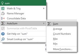
Simply type in what you want to do. For example, find the sum of cells.
As you can see in the snapshot below, a dropdown menu appears. By selecting AutoSum>Sum, we can complete the calculation right there from the menu. There's no longer a need to search help files or watch a video.
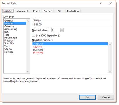
In the snapshot below, we wanted to format the cells.
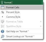
The Tell Me box takes us to the Format Cells dialogue box.