Whenever you use a function, you only have to supply the values that the function will use. These values that you supply are called arguments of the function. Excel does the rest for you.
Functions, just like formulas, always begin with an equal sign (=). After the equal sign, you enter in the name of the function. It doesn't matter if you enter it in uppercase or lowercase. Following the name of the function, you provide the arguments of the function. Arguments are always enclosed parentheses.
There are just a few things you need to remember before starting to insert functions into your spreadsheets:
1. When typing a function into a cell, don't insert spaces between the equal sign, function name, and arguments.
2. If you're adding more than one value, separate each function with a comma.
Below is an example of a function we typed into a cell:
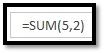
The function was SUM. The arguments were 5 and 2. We hit Enter, and Excel calculated the function for us:

We could have also entered it in as =5+2. This would have been a regular formula. Instead, the function we used was the SUM function. The values used were 5+2.
Inserting Functions into Cells
To insert a function directly into a cell, click the cell where you want to insert the function. Next, go to the Formulas tab, then click Insert Function.

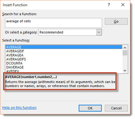
When you click Insert Function, you'll see this dialogue box:
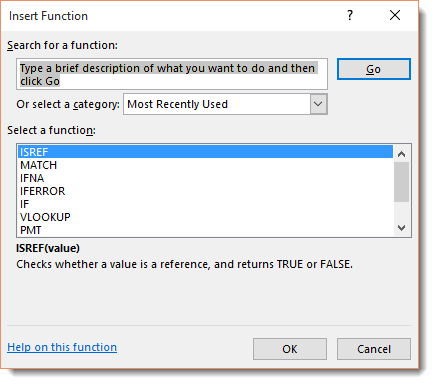
The great thing about using functions in Excel is that you don't have to know the function to get started. All you have to know is what you want to do, such as average a column of numbers.
In the Search for a Function section of the above dialogue box, you can type in a description of what type of function you want to use. We typed in Average of Cells. Click Go.
In the "Select a Function" field, Excel provides a list of functions that relate to what you entered into the "Search for a Function" field.
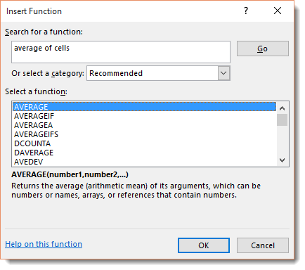
In the Select a Function field, you can click on different functions to see what calculations they perform. We already clicked on "AVERAGE". In the snapshot below, you can see what calculation it performs.
Now that you know how to insert a function, let's insert a function into an actual spreadsheet.
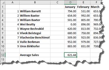
Click Cancel to exit out of the Insert Function box � if you're following along � and take a look at our sample worksheet in the following snapshot.
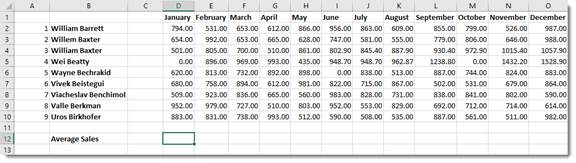
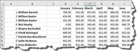
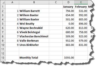
We want to determine the average sales for the month of January. As you can see, we've created a row for the average sales. We want the average sales for January displayed in D12.
To do this, we are going to click Insert Function on the Ribbon under the Formulas tab. Once again, we enter "average of cells" in the "Search for a Function field," then click the Go button.
Select Average, then click OK.
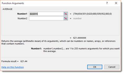
Excel prompts us for our arguments. The arguments are the cells or values that we want to use to calculate the function. As you can see, Excel entered the values for us, but we can change those by going to the worksheet and selecting the cells � or editing the values in the dialogue box.
Click OK when your values are added.
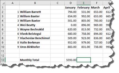
As you can see, the average sales for January was entered into D12.
NOTE: You can also insert a function by clicking  on the Formula Bar.
AutoSum
PCMag.com defines the AutoSum as a "function in a spreadsheet program that inserts a formula in the selected cell that adds the numbers in the column above it."
In other words, if we select sell E13 in the worksheet below, the AutoSum feature will add the numbers in the cells above it that are still in the same column.

To use AutoSum in Excel, go to the Editing group under the Home tab on the Ribbon.
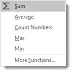
As you can see, you can use this tool to calculate the SUM, AVERAGE, COUNT, MAX, or MIN.
-
SUM is the sum of the values.
-
AVERAGE is the average of all the values in the cells.
-
COUNT counts the number of cells that contain numbers.
-
MAX is the largest value.
-
MIN is the smallest value
It can also select the most likely range of cells in a column or row that you want to use as the argument, then enters them for you.
You don't have to do anything to use the SUM feature of AutoSum but select the cell. If you want to use AVERAGE, COUNT, MAX, or MIN, you need to select them from the dropdown menu pictured above.
Let's calculate the sales total for column E in our worksheet.
As you can see, we selected cell E13 in our worksheet. This is where the sales total will appear.
To add the sum of all the values above cell E13, we go to the Home tab, then click the AutoSum button.
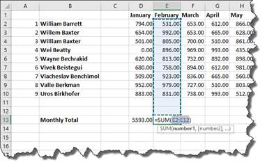
Excel automatically selected the range of cells we want to use in the argument, then entered the arguments into our function.
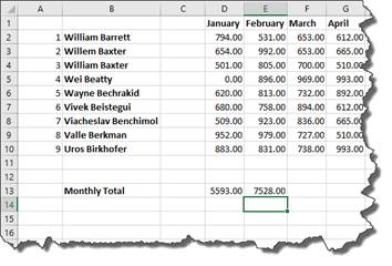
Hit Enter.
The total appears in cell E13.
If you want to edit the argument before pushing Enter, you can do that.
Locating the Function You Need
Finding the function you need can seem a daunting task. Of course, you can insert a function by using the Ribbon or Formula Bar, but you can also go to the Function Library under the Formulas tab.
In the Function Library, functions are broken down into categories.

Let's say we want to look for a function in Lookup & Reference.
Click the downward arrow. You'll see all the functions that you can use under this category.
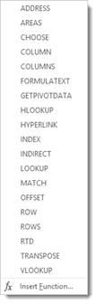
You can click on any one of the functions, and the arguments dialogue box will appear so you can enter your arguments.
You can also click Insert Function at the bottom of the dropdown menu.
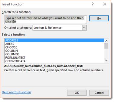
All the Lookup & Reference functions are displayed. Choose the one you want, and click OK.
References
A reference simply tells Excel where to find the information you want to use in a formula. As you've already learned, by default Excel uses the A1 reference style, or coordinate system, to identify cells. You can use these coordinates for references or you can use labels and names.
Using labels and names makes it easier to understand the information you are entering into the formula. For instance, the formula "=SUM(WednesdayTotal)" is easier to understand than "=SUM(E4:E6)
Using Names as References
As you learned earlier, a label is used to identify a range of cells such as a column or a row. You can also create a name to represent a cell or a range of cells for quicker reference in a formula. Names can also represent an unchanging number (called a constant) or even a formula.
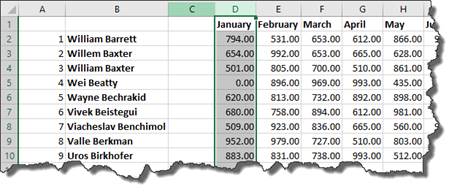
In the snapshot below, we want to name the column January as "Friday." This way, when constructing formulas, we can simply enter in Friday instead of a range of cells.
To do this, we're going to select the column "January".
Next, we go to Formulas tab, then the Defined Names group.
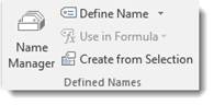
Click the dropdown arrow beside the Define Name button.
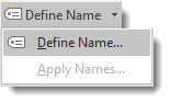
Select Define Name.
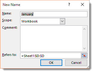
We want the name to stay the same as our label January. If we didn't, we'd enter a new name in the Name field, then the scope -- if we want it to apply to the entire workbook or just the worksheet -- then any comments we want to add.
Click OK.
Now we've named this column.
Instead of having to write out the formula as =SUM(D2:D10), we can simply enter in =SUM(Friday), then hit Enter. The calculation appears in the cell.
Now let's create a name for a constant. In this example, we'll say it's sales tax.
Click in an empty cell, then go to Define Name.
Give it the Name: SalesTax.
The scope is the workbook.
In the Refers To section, we want to enter .08.
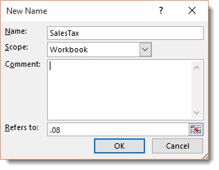
Click OK.
To see all the names you've created if you need a reminder, click the Names Manager in the Defined Names group.
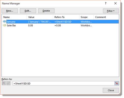
In the dialogue box above, you can add, edit, or delete names.
Now, let's go back to the SalesTax name for a minute. We now have a reference for sales tax. We can then use that reference in a formula. In the example below, we'll apply sales tax to the total for January, which is cell D13.
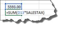
As you can see in the formula above, we entered the function SUM, then included the values used for the function in parentheses. These values were from D13 and the SALESTAX reference.
Hit Enter.
We now get the amount of sales tax.

We can now add (SUM) the amounts from D13 and D14 together to get a grand total.
Absolute, Relative, and Mixed Cell References
There are two kinds of cell references: Absolute and Relative.
A relative reference in a formula depends upon its position in a worksheet. For instance, the cell coordinates in the following example "B4:B6" are relative references.
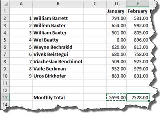
In the example below, we can copy the formula in cell D13 and paste it as a formula into cell E14.
When we do this, the formula stays the same, but the relative references change.
We'll show you how to copy and paste formulas in just a minute.
For right now it's important to realize that the formula stayed the same, but the relative references changed because Excel recognized the relationship between the formula in cell D13 and its cell range (D2:D10). When we pasted the formula into a new cell, it created the same relationship in the new position.
That's a relative reference.
An Absolute Reference does not depend upon its position in a worksheet. For instance, if the value in cell D13 were an absolute reference, when we pasted the formula in cell E13, the formula would read: =SUM($D$2:$D$10).
The symbol "$" in cell coordinates tells Excel that this is an absolute reference. To create an absolute reference, type a dollar sign before the column reference and row reference in the formula.
A mixed reference contains both an absolute reference and a relative reference. Which means, it can either contain an absolute column and a relative row, or a relative column and an absolute row.
Copying and Pasting Formulas without Relative References
At some point when using Excel, you may want to copy a formula, then paste it into a different cell, as we did in the last section.
Let's use the same example again.
We want to use the same formula in cell E14 as we did in D13. This formula calculates sales totals by month.
To do this, we are going copy the formula in cell D13 and paste it as a formula into cell E14.

We start out by selecting cell D13, right clicking, then choosing Copy from the context menu.
Next, we click cell E13 to make it active, right click, then either click on the Formulas icon, as highlighted below.

Or by clicking on the arrow beside Paste Special and selecting Paste Special.
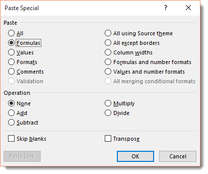
Select Formulas, then click OK.
As you can see below, the total for February then appears in cell E13.

The formula remained the same. Only the relative references changed when we pasted the formula into cell E13.
Now let's change it to absolute references.
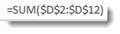
We don't want the references to column D to change, so we add a dollar sign before the column and row in cell D13.
Now, we can click on cell D13 in our worksheet. You can either click Copy under the Home tab in the Clipboard group, of you can right click and select Copy.
Now click on the cell that you want to paste into. For us, it's E13.
Right click and select Paste Special>Paste Special.
We want to paste the formula.
Click OK.
As you can see, our formula with our absolute values appear in cell H8.
If you don't add absolute values to your formula in the cut/copied cell, it will change the cell references to the pasted cells coordinates, as mentioned above.
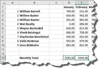
Copying and Pasting Only Values from One Cell to Another
You can also simply paste the calculation and value from a formula in one cell into another.
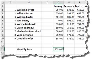
Let's reuse our example from the last lesson, but instead of copying the formula, let's copy and paste the value.
Copy cell D13 again.
Next, go to cell E13 and right click, then choose Paste Special>Paste Special.
In the Paste Special dialogue box, check Values.
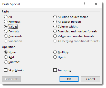
Click OK.
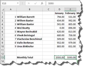
You can look in the Formula Bar with cell E13 selected and see that only the value was pasted, not the formula.
Linking Formulas
When you paste a formula, you may want to link back to the cell where you copied the formula. There may be data there that needs referenced, etc.
For example, you may have one table in a worksheet that lists your employee's sales figure by the month, then presents a grand total of sales by all employees for each month of the year.
However, you may also have another table in your worksheet that deducts total expenses for each month from the monthly sales figures in order to determine profit. You may want to use the formula you placed in a cell to calculate the grand total of sales for the month of January in the other table so you deduct expenses from that amount. The easiest way to do that is to link formulas.
To link formulas, first select the cell that contains the formula that you want to copy. In our example, it's cell D13 since that contains the sales total for January. We want to link to the formula instead of simply copying and pasting the formula or the calculation. We want to link to it so if the values change in the formula in cell D13, it will also change in our other table where we are using the formula.
We want to move the formula from D13 down further on our worksheet where we subtract expenses.
Here's where we subtract expenses in our worksheet:
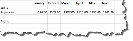
As you can see, we have the expenses entered for each month. Now all we need are the sales totals. We want to fill in January sales with the calculation from D13.
To do this, we start out by copying D13.
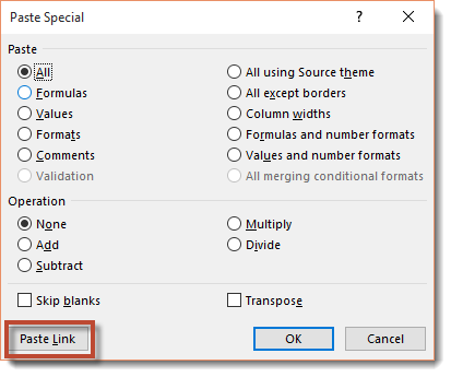
Next, we go to the cell in our other table that represents total sales for January. This is cell C22. Right click on it, and choose Paste Special>Paste Special.
Click the Paste Link button.
As you can see, the calculation is now pasted into cell C22.
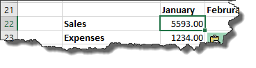
Now, if you look at the Formula Bar whenever you click on cell C22, you'll see it links you to cell D13.

Notice the references were changed to absolute.