Although Excel is well known for its mathematical capabilities and features, it also has some powerful tools for creating text formulas to manipulate text.   We are going to take this article to learn some of the text functions and formulas, then teach you how they are used. More specifically, we will show you how to use them.

The LEFT and RIGHT Functions

Two of the common text functions you will come across in Excel are LEFT and RIGHT. These functions are used to extract text data from a worksheet.

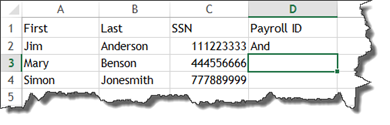
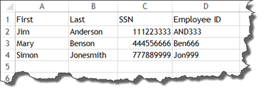
For example, it is not uncommon for businesses to use the first three letters of an employee's name for identification purposes and payroll. Someone with the last name Anderson might be listed as AND followed by the last three digits of their social security number.   They may be listed for payroll purposes as AND325.  

We can use the LEFT and RIGHT text function to extract the first three characters of their last name.

Let's take a look how it works by looking at the worksheet below.

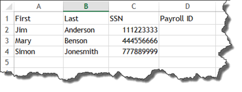
We are going to use the LEFT function to extract the first three letters of each employee's last name.

We start a text function the same way that we start a mathematical function.

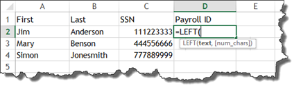
We can now see the parameters, which are the text which we wish to use, then the number of characters we want to appear. 

Select the cell that contains the text, followed by the number of characters.

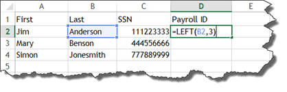
Press Enter.

The first three letters of the last name are now in the cell.

We will show you how to combine that with the last three numbers of the social security number later in this article.

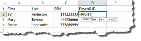
For now, let's now look the RIGHT function.   The RIGHT function extracts characters from the end of text. So, instead of the first three letters of the last name, it will be the last three letters. 

We start out by entering the equal sign, then RIGHT.

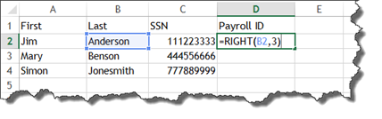
As you can see, the parameters are the same as with the LEFT function.   Select the cell that has the text, then the number of characters you want to extract from the end of the name.

Press Enter.

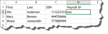
The LEN and TRIM Functions

Now that we have covered the LEFT and RIGHT functions, let's talk about two more text functions. These are the LEN and TRIM functions.

Sometimes when you import data into Excel, there can be spaces at the end of data in a cell that you can't see. 

If you are trying to use the RIGHT function to extract the last four letters of text, you may end up seeing something like this in your worksheet:

Even though we have used the RIGHT function to extract the last four letters of the text string, you can see that some cells only have three letters in them.

There is a reason for this.

When we imported the data into Excel, there were some spaces at the end of some of the strings of text.   So, when the RIGHT function counted four characters from the right, it also counted a space that we did not know was there in two instances in our worksheet.   That is why only three characters are showing.

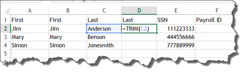
When you import data into Excel, it is typically best to use the TRIM function for cells that contain text. That way, if you want to manipulate that text later using either the RIGHT or LEFT function, the spaces will no longer be there.

That said, we use the TRIM function for text data that we imported.  

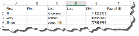
As you can see above, we have added two new columns to do just that.

Let's enter the trim function. It only requires one parameter, which is the text.

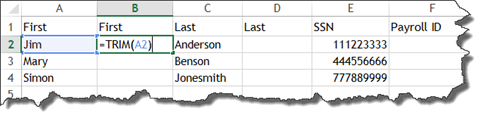
Press Enter.

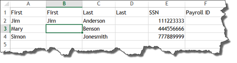
The employee's first name appears. However, there are no invisible spaces. 

Return to the cell where we just added the TRIM function. Drag the handle in the cell to finish out the column.   Then, let's do the same with the Last column.

Press Enter, then select the cell again and drag the handle to finish the column.

However, now there is a problem. We have two columns for both the First and Last name. If we try to delete the columns that contain the imported data, since we do not need them anymore, we will get #REF errors.   We could enter the names instead of cell references, but that would be a lot of work. All names would have to be entered individually.

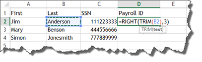
Instead, the best way to do this is NOT to create the two extra columns, but instead embed the TRIM function in with the RIGHT function. 

In our worksheet below, we have added the RIGHT function and told Excel we want the last three characters of the last name.   Then we embedded the TRIM function so that all spaces at the end are trimmed off. 

Once you enter TRIM(B2), Excel takes you back to the RIGHT function and prompts you for the num_chars parameter. 

The LEN function tells you how many characters are in a string. LEN is short for length.

Let's see how many characters there are in the last name Anderson.

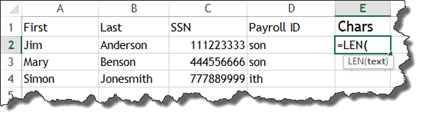
As you can see, it only requires one parameter. We are going to click on cell B2.

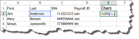
Press Enter.

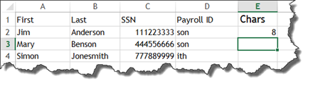
We can see that there are eight characters in the last name Anderson.

Take a look at the worksheet below.

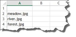
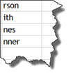
As you can see, we have a list of image file names.

We want to remove the .jpg from the end so only the name of the picture shows up in the next column.

We will use the LEFT and LEN functions to do this.

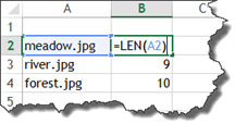
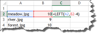
The first thing we are going to do is determine the length of each file name by using the LEN function.

Next, we are going to use the LEFT function and enter the text parameter.

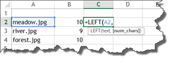
For the num_chars paremeter, we are going to enter the length found in cell B2 and subtract the number of characters in .jpg, which is 4.

Press Enter.

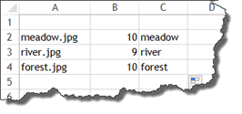
We now have our image file names without the .jpg after them.

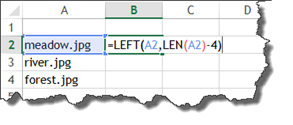
If we did not want to have a column for length in our worksheet, we could simply embed the LEN function in with the LEFT function, as shown below.

The FIND and MID Functions

The FIND function gives you the start position of one text string within another, then displays a number which represents the character from which the searched string starts.   The MID function lets you extract text from the middle of a string and continue for a specified number of characters.

Let's learn how both functions work, starting with the FIND function.

Look at the example below.

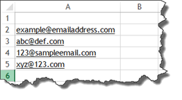
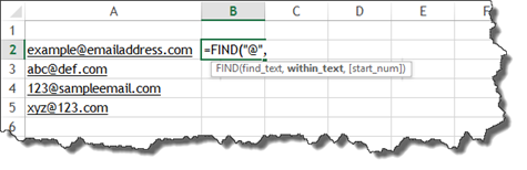
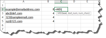
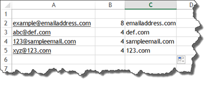
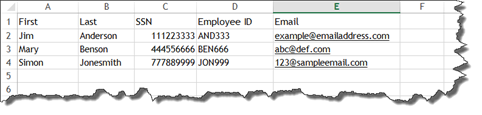
As you can see, we have a list of email addresses. We want to extract the domains from the list in order to find out which domains our friends are using.

To do this, first we have to use the FIND function to 1. Find the @ sign, 2, determine where it occurs in the string. For example, the third character of the string.

We will use the FIND function.

Let's start the function.

Now we can see the parameters for the formula.

First, we need to tell Excel what text we want to find.   We want to find the "@" sign within the email address.

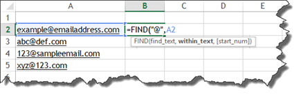
The next parameter, within_text, is asking where Excel needs to look for the text.  

We select the cell that contains the email address.

The parameter start_num is optional. You would use it to tell Excel to start searching at a certain number of characters into the string. If you are looking for several instances of the character, it is helpful to use.

We do not need to do that, so we add a closing bracket.

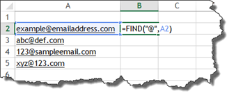
Press Enter.

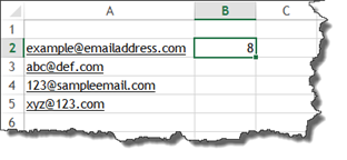
Our @ occurs eight characters into the string.

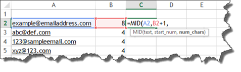
Next, we are going to use the MID function to extract the domain that comes after the @ symbol.

Let's start the MID function

We can now see the parameters.

The first parameter is the text that we want to manipulate.

This is the cell that contains the email address.

The next parameter is the start_num.   This is the number of the first character that we want to extract. That character will be the first one after the @ sign. We want one more than that.

Finally, num_chars is the number of characters that we want to extract from the string. Since everyone's domain name has a different number of characters, this is impossible to know. 

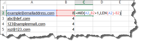
To figure this out, we will embed a LEN function, as you can see above.   In order to find out how many characters we need to extract, we will subtract the number of characters BEFORE the @ sign from the number of characters in the email address.    This will leave us with the number of characters that remain after the @ sign.

Press Enter. You can now see the domain.

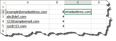
Drag the handle in the results cell to finish the rest of the worksheet.

The CONCATENATE Function

In the first section of this article, we mentioned that it is not uncommon for a business to combine the first three letters of an employee's last name with a string of numbers to come up with an employee ID. 

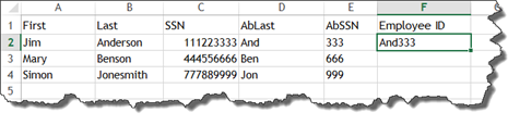
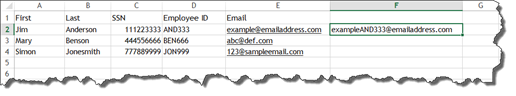
In our worksheet below, we have a list of employees with their social security numbers.   We also used the LEFT and RIGHT functions to extract the first three characters from their last name, and the last three numbers from their social security numbers.

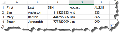
What we want to now do is combine the characters in the AbLast column with those in the AbSSN column. 

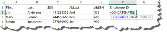
We will do this using the CONCATENATE function.

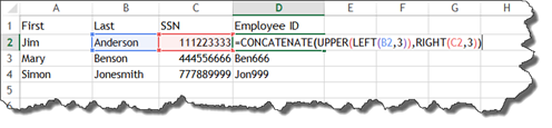
In the snapshot below, we have started to add our function.

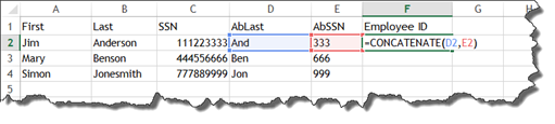
Now, we select the text that we want to use for the function. We want to combine cells D2 and E3.

 Press Enter.

If we wanted to add a space between the two different strings of characters, we would add spaces between the cells in the formula by using a quote, a space, then another quote.

That said, if we did not want to have to add columns D and E to our worksheet, we could embed LEFT and RIGHT functions within the CONCATENATE function.

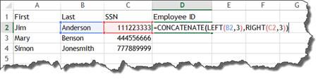
Press Enter.

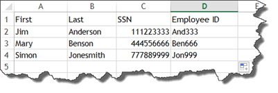
You can then complete the worksheet.

The Changing Case Functions

Using text functions, you can change your text to uppercase, lowercase, or title case. 

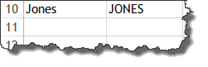
To change text to all uppercase, use the UPPER function, as shown below.

Press Enter.

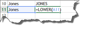
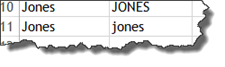
To change it to lowercase, use the function LOWER.

Press Enter.

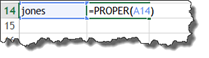
To change it to title case, use the PROPER function.

Press Enter.

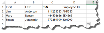
Now, let's go back to our employee ID's.   We want to make the first three letters of the employee ID all uppercase. To do that, we have to embed the UPPER function.

Press Enter.

Now we can drag the handle in D2 to finish the worksheet.

The REPLACE and SUBSTITUTE Functions

The REPLACE and SUBSTITUTE functions are a lot alike; however, they are not exactly the same thing.   To show you what we mean, we are going to show you how each of these functions work.

In our worksheet below, we want to use the REPLACE function to add the employee ID after the first part of the email address.

To do this, start the REPLACE function.

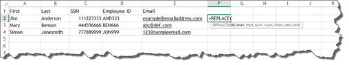
The first parameter is old_text, or the cell that contains the text we want to manipulate.  

The start_num is where we want to start adding the new text.   This would be the @ symbol for all email addresses, so we use the FIND function to find it.

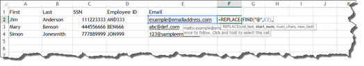
The parameter num_chars asks for how many characters we want to replace. We do not want to replace any, so we put zero.

The new_text is the new text we want to add.   That is the employee ID.

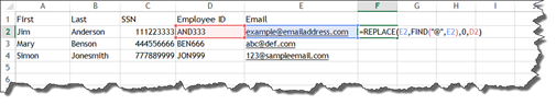
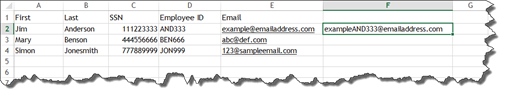
Press Enter.

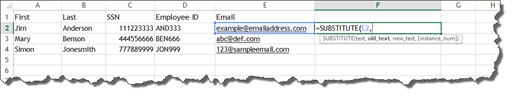
The SUBSTITUTE function can be used to get the same result.

Let's start the SUBSTITUTE function.

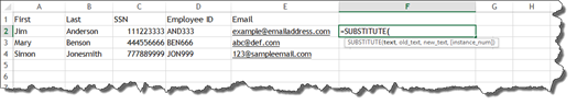
First, we want to enter the text we want to manipulate. For this example, it is the email address.

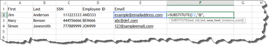
Next, we enter the old text that we want to replace with the new text. We will enter the @ sign.

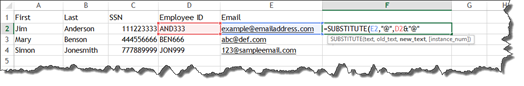
Now we enter the new text we want to add. This is the employee ID as well as the @ symbol. We have to add the @ symbol back to the email address. We use the cell reference, an ampersand, and the @ symbol to do this.

The parameter instance_num is optional. It wants to know which instance of the @ symbol we want to replace. Since it only appears one time, we do not need to worry about this.

Add the closing bracket.

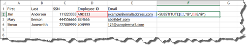
Press Enter.

The CHAR Function

The CHAR function lets you add characters to a string that are not on your keyboard. In addition, it allows you to add carriage return to strings.   For example, you can add a carriage return to an address to break it up into two lines.

Take a look at our worksheet below.

We want to combine these two strings into one, then add a carriage return.

To do this, we would start by using the CONCATENATE function. 

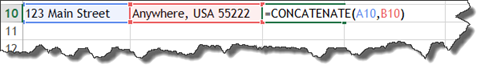
Now we need to create a carriage return between A10 and B10. To do this, we will use the CHAR function.

With the CHAR function, we add a number between 1 and 255 to get the character we need. 

We need a carriage break.   This is number 10.

You can see that we inserted the CHAR function between the two cell references – which is where we want our line break.

Press Enter.

Since there are 255 different characters that you can insert with a CHAR function, it is impossible to list them all in this article. 

Formatting Date and Numbers Using the TEXT Function

We already know how to format dates, texts, and numbers in cells using Excel. That is easy enough to do without a function.   However, we cannot format a date or text if a cell contains both.

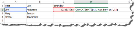
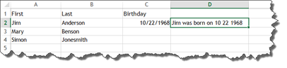
For example, in our worksheet below we have used the CONCATENATE function to put Jim's name, then his birthday.

Press Enter.

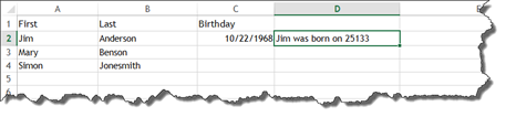
As you can see, Excel entered a number instead of the birthdate. This number is the count of days since Excel's beginning count date. This date is January 1, 1900.

To format the date, we will use the TEXT function.

We will insert it before the date in the formula.

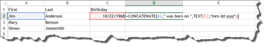
As you can see, we use MM DD YYYY to tell Excel which date format to use. If we wanted to write out the month, we would have entered MMMM DD YYYY. 

 Press Enter.

To format numbers with the TEXT function use zeroes and commas, if needed. For example, 20,000 would be 0,000 in the TEXT function.

Preserving String Values

In this article, we have learned to use functions to manipulate text. We have created several cells with functions in them that extract and combine text. This is great as far as our worksheet goes, but the problem comes if you need to copy and paste a column that you have created using these functions into another worksheet. You will get #REF errors.   This is because we are pasting a relative path. 

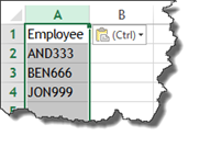
In the worksheet below, we tried to paste our employee ID column into a new worksheet.

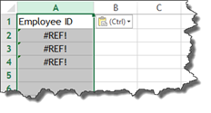
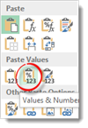
You can see the #REF errors that we have. To fix this, click the downward arrow to the right of CTRL in the spreadsheet. Choose Values & Number Formatting from the Paste Values section.

You can see that our employee ID's now appear.