With all the functions and formulas Excel 2016 allows you to use in worksheets and workbooks, there is little doubt that you are going to have some errors.   If you have a lot of data contained in your worksheets and workbooks, it can be a chore to go back and isolate each error, then take steps to fix it. Finding and fixing errors could wind up being just as time consuming as entering and calculating the data. At least, it would be if Excel 2016 did not offer you the tools you need to help you efficiently audit and troubleshoot your workbooks and data.

About Tracer Arrows

Tracer arrows allow you to trace problems in a worksheet. If there are errors in formulas or things are not working as they should within your worksheet, tracer arrows can help you find the problem. They do so by helping you trace "the path" of your data.   Tracer arrows show you how data in one cell is connected to data on other cells. 

In Excel 2016, there are two different types of tracer arrows.

• Dependent tracer arrows show you which cells are dependent upon the value in the cell you have selected.  They show you the cells that come AFTER the cell you have selected and our dependent on the data from the cell you have selected. 

• Precedent tracer arrows work in the opposite way. They show you what cells feed into the cell you have selected. The cell where the arrow starts is the first cell that feeds into the cell you selected.   The arrow ends in the cell you selected.

Adding or Removing Tracer Arrows

Adding and removing tracer arrows is easier than it may sound.   We are going to first cover how to add dependent tracer arrows, followed by precedent tracer arrows, as well as how to remove them.

Take a look at our worksheet below.

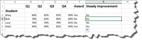
We want to find out which cells are dependent on G4.

To do this, we are going to go to the Formulas tab. 

Go to the Auditing section, and click Trace Dependents.

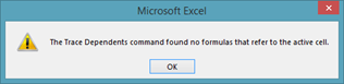
As you can see, we get a message that there are not any formulas that refer to the active cell.

Instead, let's click on cell B3, then click Trace Dependents.

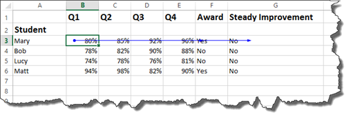
We can now see all the cells that are dependent on cell B3. Since we created this worksheet, we know that there are formulas who rely on the data in cell B3 to perform their calculations.

To remove a dependent tracer arrow, go to Remove Arrows in the Auditing group under the Formulas tab and click the downward arrow beside it. From the dropdown menu, choose Remove Dependent Arrows. 

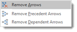
If you select Remove Arrows, it will remove both Dependent and Precedent arrows.

To add a precedent tracer arrow, click on a cell. Remember, Excel will show you all cells that feed into the one you have clicked.

We are going to select G4 again.

Go to the Formulas tab. Click Trace Precedents in the Auditing group.

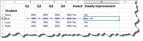
You can now see which cells feed into cell G4.

To remove a precedent tracer arrow, go to Remove Arrows in the Auditing group under the Formulas tab and click the downward arrow beside it. From the dropdown menu, choose Remove Precedent Arrows. 

Using Error Checking

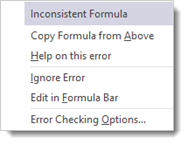
Excel gives you quite a few ways to audit your worksheets and check for errors.   The first way is using Error Checking. Error Checking points out all of the errors that may occur in cells or formulas in cells, then allows you to get help with the error, ignore the error, copy the formula from the cell, or edit the formula in the Formula Bar.

To use Error Checking, go to the Formulas tab, then click the downward arrow beside Error Checking in the Formula Auditing group. Select Error Checking

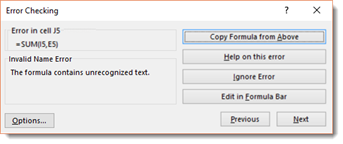
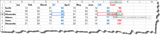
As you can see, Excel pulls up the first cell where there is an error.   It tells us the error exists because of an inconsistent formula.   If we look in our worksheet and pull up the cell above it which uses the same formula, we can see there is indeed an error. The sum should be calculated for E5,I5. Instead, it is showing as I5,E5.

Let's go back to Error Checking.

If we click on Copy Formula from Above, it will copy the formula from the cell above it.

This fixed our error. 

For the time being, however, we are going to reproduce the error to show you what your other options are with Error Checking.

This time, let's click on Help On This Error.

The Excel 2016 Help files will open.

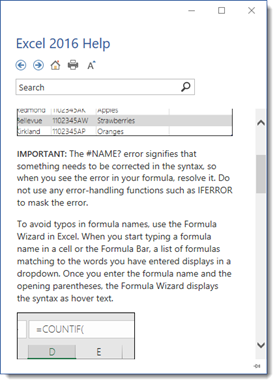
This is very generalized help about using Error Checking in Excel.

The next button we are going to explore in the Error Checking dialogue box is Ignore Error.  

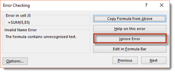
If you click this button, the error will be left in the worksheet.

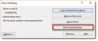
The final button is Edit in Formula Bar. This enables you to correct the formula in the Formula Bar.

If you click the Next button, it will take you to the next arrow in the worksheet.

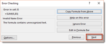
We are going to click the Copy Formula from Above button again to fix the error.

Finding and Correcting Circular Reference Errors

In Excel 2016, a circular reference is an error that occurs when a cell is dependent on itself to calculate a formula, so it is unable to display the result of the calculation in the cell.

Here is an example. We want to add B2 plus C2.   We have placed the formula inside C2, which means C2 is where we want the result displayed.

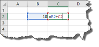
When we push Enter, look at what happens.

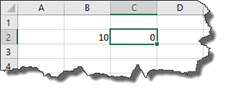
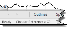
A zero appears in the cell. At the bottom left corner of the spreadsheet, we see that a circular reference has occurred.

 We can also go to Circular References in the Error Checking dropdown menu under the Formula tab.

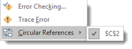
NOTE: Whenever you error check an Excel worksheet, you can go to the Formulas tab, then click the Error Checking dropdown menu to check for circular references. As you can see above, Excel will show you where there are circular references in your worksheet.   You can click on any that are listed, and Excel will take you to them.

If we click on $C$2, we are taken to our cell.

We can then click the green pop out signal in the upper left hand corner of the cell. It looks like this:

We are offered options to correct the error.

The options we see in this dropdown menu are the same that we encountered in the last section using Error Checking.  

We are going to choose to Copy Formula from Above, and the error is fixed.

Trace Error

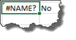
Whenever we see an error in a cell such as #VALUE and #REF, as shown below, we can easily enough fix these types of errors by going to the Error Checking dropdown under the Formulas tab and selecting Trace Error.

This will make either a precedent or dependent trace arrow appear in the worksheet.

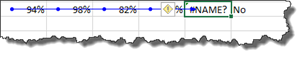
In the snapshot above, we have a precedent tracer arrow. We know this because the arrow starts in a cell, then ends in the cell where there is the error.

The precedent tracer arrow lets us know that we may need to check those cells when fixing the error. Once you find and fix the error, the precedent tracer arrow disappears.

Formula Processing

If you have a long formula in Excel, it can be hard to go back and see exactly what the formula is actually doing. 

Take a look at the formula below.

In this formula, you can see that we have a lot going on. We have more than one calculation, plus we have a lot of cell references like C6 and B6.

If we want to see exactly what is going on in the formula as Excel processes the formula step-by-step, we go to the Formulas tab, then click Evaluate Formula in the Formula Auditing Group.

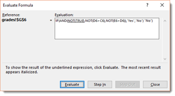
We then see this dialogue box:

In the dialogue box, we see our formula.   We also see part of the formula is underlined. Click the Evaluate button.

Excel now evaluates the part of the formula that was underlined. We see the data that is in the cell now instead of just the cell reference.

Click the Evaluate button again.

We now see the next thing that is going on in the formula. Again, we see the actual value instead of the cell reference.   In addition, what you are seeing in the Evaluate Formula window is the steps Excel takes to process the formula.

Click Evaluate.

We can go through like this and evaluate each part of the formula to see what is going on.

If you click the Step In button, Excel will step in to the part of the formula you are looking at, as shown below.

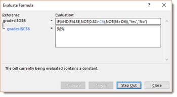
The top field shows us that we have stepped in to C6.

The bottom field shows us that the value in C6 is 98%.

You can then click Step Out and keep evaluating your formula.

As you evaluate your formula by clicking the Evaluate button, you are also watching the steps Excel takes to process your formula.  

As you can see in the snapshot below, Excel has processed and calculated the formula.

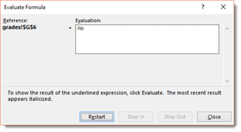
Click the Restart button to evaluate the formula again, or click Close.

The Watch Window in Excel 2016

The Watch Window in Excel 2016 lets you watch particular cells to see if the value in those cells change.

To access the Watch Window, go to the Formulas tab, then click on Watch Window.

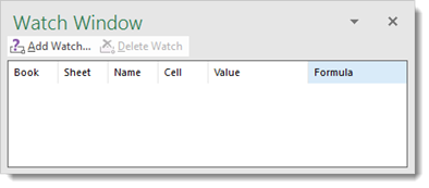
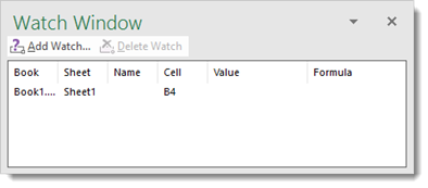
As you can see about, the Watch Window tells you the workbook and worksheet where the cell is located, the name, the actual cell that is being watched, the value of that cell, as well as the formula contained in that cell.   

This allows you not only to watch a cell, but also know exactly where the cell is located, as well as its purpose (for example, to calculate an average).

Because the Watch Window lists workbooks as well as worksheets, you can keep watching cells as you work in other workbooks.   If the data in a watched cell changes, you will see it in the Watch Window.

You can move the Watch Window around Excel and dock it above, below, or to the side of your worksheet.

This can be helpful as you are checking your workbook for errors.   You can use the Watch Window and see as those errors are being fixed.

The Watch Window is also helpful if you have a formula that uses cells from other worksheets in its calculation.    As you change values of the other cells that feed into the cell you are watching, you can see the value of the watched cell change in the Watch Window.

To add a cell to watch in the Watch Window, select the cell, then click Add Watch in the Watch Window.

You will then see the address of the cell in the Add Watch dialogue box.

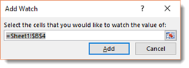
Click Add.

You can then see that cell in the Watch Window.

Creating and Running Macros

The best way to teach you how to create and run a macro is to walk you through it step by step.

In the worksheet below, we have simply listed the tasks that we want our macro to perform.

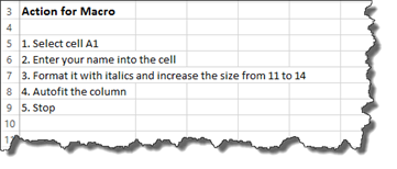
We are going to create a macro that selects sell A1, enters our name into it, makes the font italic and increases the size to 14, then uses autofit to determine the column size.

Notice that #5 is telling the macro to stop.   This is important. You record a macro. Just as with anything you record, you must tell it to stop.

Let's create the macro.

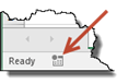
To record a macro, you can go to the Developer tab and click Record Macro, or you can go to the bottom of your worksheet and click the button to the right of the word Ready. It looks like this:

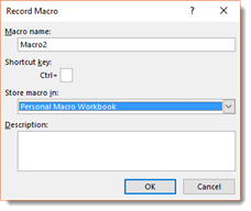
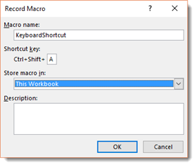
You will then see the Record Macro dialogue box.

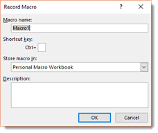
First, give your macro a name in the Macro Name field.   You can name your macro anything you want; however, the name cannot contain spaces.

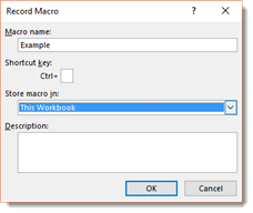
Next, we can tell Excel what keyboard shortcut to use.   We are not going to fill that in right this second. Instead, let's move on to the next field.

In Store Macro In, you have three choices.

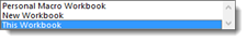
Out of these three choices, there are only two that you need.

• Personal Macro Workbook stores the macro with your machine.   We will talk more about this later in this article.

• This Workbook stores the macro with your current workbook.  If you send the workbook via email to someone else, the macros will be there for them to use.

We are going to choose This Workbook.

Next, enter a description for your macro.

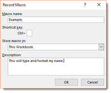
Click OK. 

When you click OK, the recorder starts to run.

If you look at the ribbon under the Developer tab, you can see that it says Stop Recording where the Record Macro button was before you clicked it.

To the right of the word Ready, you will see a white square that looks like a Stop button on a tape recorder.

You can click either one of these things to stop recording your macro.

Now, you can start recording your macro by performing the actions we listed.  

Take your time when you record your macro. If you make a mistake, even if you undo it, Excel records that mistake.   Excel does not record the time it takes for you to enter your macro though.   That said, it is important that you take your time.

Record your macro, then press Stop Recording.

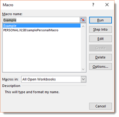
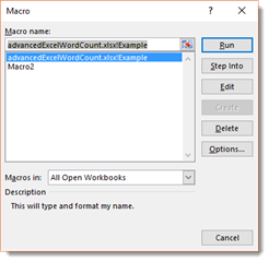
To make sure your macro recorded or to access your macro, go to the Developer tab again. Click the Macros button.

Our macro, Example, is now shown in the list.

If you want to run the macro, click the Run button.

Saving a Workbook with Macros

It is very important when you save a workbook that contains macros, that you save them as macro-enabled workbooks. If you do not save them as macro-enabled workbooks, the macros will not be saved.

To save a workbook with macros, go to File>Save As.

In Windows 8, choose the location where you want to save the workbook.

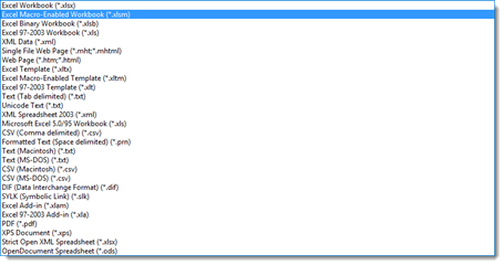
In the Save as Dialogue box, go to the Save as Type field and choose Excel Macro-Enabled Workbook, as highlighted in blue below. 

Notice that macro-enabled workbooks have a different file extension. It is .xlsm.   A workbook without macros is .xlsx. 

You can then name your file, and click the Save button.

Macro Security Settings

Now that we have saved our macro-enabled workbook, we also need to set the security settings for our workbook since it has macros.

To do this, we will go to the Developer tab again. This time we will click the Macro Security button. 

This takes us to the Trust Center and automatically opens it with the Macro Settings tab selected.

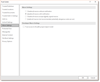
Under Macro settings, you can establish the security settings.

By default, Disable All Macros with Notification is checked. You want to leave this checked. Whenever you open a workbook that contains macros, you will be asked if you want to enable the macros.

Click OK.

When you save and close a workbook, then reopen it, you will see this message above your worksheet.

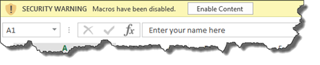
Click the Enable Content button so that you can use the macros in the workbook.

Once you enable the content for a workbook, you will not see the security warning again for that workbook. The content will automatically be enabled.

The Personal Macro Workbook

The personal macro workbook does not exist until you create it.   You create a personal macro workbook when you create and save your first workbook, choosing to save it to your personal macro workbook.   Each time you open Excel, the macros you created in your personal macro workbook will be there for you to use. Your personal macro workbook will be available to you no matter what Excel workbook you open – as long as you open it on the machine where you created the personal macro workbook.

For example, if you create the personal macro workbook on your desktop computer that you have at home, the macros that you save to that personal macro workbook will be available to you. It does not matter what workbook you created them in. They will be available in all workbooks that you open while on your home desktop computer.

However, if you use your laptop or a computer at the office, the personal macro workbook, as well as the macros, that you created on your desktop computer will not be available to you.   Your personal macro workbook and all the macros included in it are machine specific.

That said, when you open your macros, you will be able to distinguish macros that are part of your personal macro workbook from macros that are workbook specific.   The macros that are part of your personal macro workbook will have PERSONAL.XLSB! in front of the macro name, as shown below.

To create and store a macro in a personal macro workbook, click Record Macro under the Developer tab. 

In the Store Macro In field, select Personal Macro Workbook from the dropdown menu.

When you store a macro in your personal macro workbook, Excel will confirm that you want to save that macro in your personal macro workbook when you try to exit Excel.   This only happens the first time you exit Excel after storing a macro in your personal macro workbook.

If you click Save, the macro is saved to your personal macro workbook. 

If you click Do Not Save, then the macro will not be saved and will not be available in any workbook again.

NOTE: If you like to back up your files, the file that contains your personal macro workbook is titled XLSSTART. The path to it will always be Microsoft>Excel>XLSSTART.   Where your Microsoft folder is stored will depend on your operating system and installation. 

Deleting a Macro

To delete a macro that you have saved to a workbook, go to the Developer tab, then click on the Macros button.

Select the macro by clicking on it, then click Delete.

You will then see this message:

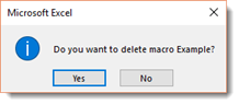
Click on the Yes button if you want to delete the macro.

If you try to delete a macro that is included in your personal macro workbook using the steps we just detailed, you will see this message:

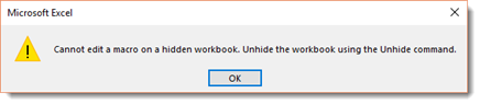
It tells you to unhide the workbook before you can delete it. Click OK.

We will show you how to unhide the workbook in a minute. For now, it is important to remember that macros stored in your personal macro workbook are stored in the PERSONAL.XLSB workbook.   When you open another workbook in Excel, those workbooks are available to you to use. However, the macros are not stored in the workbook you have opened. Again, they are stored in the PERSONAL.XLSB workbook instead. 

In order to delete a macro from the PERONSAL.XLSB workbook, you must first unhide it. 

To unhide the workbook, go to the View tab.

Click Unhide in the Window group.

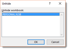
Select the workbook you want to unhide. You can see that our personal macro workbook is listed.

Click OK.

The personal macro workbook is now open on your machine.   To delete a macro from it, go to the Developer tab.

Click the Macros button.

Select the macro that you want to delete, then push the Delete button.

You will see this message:

Click Yes.

Close your personal macro workbook as you would any other workbook.

You will then see this message:

Click Save to save the changes.

The Use of Relative or Absolute Referencing in Macros

Remember, an absolute cell reference is when you want a cell reference to be fixed on a cell.   In Excel, you can mark rows and columns as absolute by adding the dollar sign ($) before either the row, column, or both when working with formulas.

A relative cell reference is a cell reference that can change when something, such as a formula, is copied from one cell to another. We have seen examples of relative references when we dragged the bottom right handle down to essentially copy a formula into different cells and complete a worksheet.

In Excel 2016, whenever you create and record a macro, the cell references are automatically absolute. If you create a macro that starts in A1, if you use that macro in a different worksheet, it will start in cell A1. It does not matter which cell is active when you run the macro, it will run in cell A1. 

When you create an absolute reference when recording a macro, you can have the macro run in any cell.   For example, you can create the macro while cell A1 is active.   When you run the macro, you can run it with cell F4 active, and the macro will run in cell F4.

To use a relative reference when recording a macro, go to the Developer tab, then click the Use Relative References button.  

Next, click the Record Macros button.

Go ahead and name the macro, then choose where you want to store it. You can also enter a description.

Click OK.

Record your macro. When you are finished, stop recording.

Now you can click on any cell in a worksheet, go to macros under the Developer tab, then run your macro.   It will appear in the cell that is active.

If you do not want future macros to have relative references, make sure you go back to the Developer tab and click Use Relative References again to turn off the use of relative references when recording macros.

Using Keyboard Shortcuts to Run Macros

Thus far in this article, whenever we wanted to run a macro, we went to the Developer tab, then clicked the macros button. However, since macros are supposed to save time and create shortcuts, this can seem like extra work that is not really needed.

Instead of going to the Developer tab and clicking Macros every time you want to run one, you can instead assign a macro a keyboard shortcut. The keyboard shortcut always involves the CTRL key, plus a letter on your keyboard. You must choose a letter. Your shortcut cannot involve numbers or symbols.

If you choose an uppercase letter, the keyboard shortcut will be CTRL+Shift+ the letter that you choose. If you choose a lower case, it will simply be the CTRL key plus the letter that you choose.

Let's create a new macro by going to the Developer tab, then clicking Record Macro.

Go ahead and name the macro.

Enter the shortcut, as we have done below.

When you are finished, click the OK button, then record your macro.

Stop recording when you are finished.

Now, whenever we want to use the macro that we just created, we can simply push CTRL+SHIFT+A.