Key Terms
o Measure of dispersion
o Variance
o Population variance
o Standard deviation
o Population standard deviation
o Sample variance
o Sample standard deviation
o Degrees of freedom
Objectives
o Use the variance or standard deviation to characterize the spread of data
o Understand the difference between measures of dispersion for populations and for samples
In this article, we will consider measures of dispersion, which describe how the data is "dispersed" around a central value. For the measures of dispersion considered, we will rely on the mean as the standard measure of central tendency, and we will consider measures for both a population and a sample (the calculation of these values differs slightly).
Population Variance and Standard Deviation
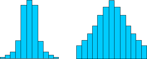
Given a population mean μ, we might also want to know how the data is distributed around that mean. One potential way to quantify this distribution is through another mean: the average distance of the data points from μ. Consider the histograms below. The histogram on the left shows data that is tightly "packed" around the mean; the histogram on the right shows data that is loosely "packed" and spread further out around the mean.
Let's explore how we can quantify this dispersion. First, we must calculate the mean μ for a population (or ![]() for a sample). Next, we want to calculate the distance of each data value from μ. Given a data value xi, a simple difference such as xi – μ would not be suitable, since the difference could be positive or negative, and summing differences of varying signs could result in canceling that improperly decreases the dispersion value. To avoid this difficulty, let's square the distance: (xi – μ)2. This removes the sign from the distance, and we can add different distances to get a more accurate value. Given a data set with N values (such as {x1, x2, x3,., xN}), we can simply find the average squared distance by adding all values of (xi – μ)2 and then dividing this sum by N. This average squared distance is called the variance (or population variance, σ2), and we can express the formula for the variance as follows:
for a sample). Next, we want to calculate the distance of each data value from μ. Given a data value xi, a simple difference such as xi – μ would not be suitable, since the difference could be positive or negative, and summing differences of varying signs could result in canceling that improperly decreases the dispersion value. To avoid this difficulty, let's square the distance: (xi – μ)2. This removes the sign from the distance, and we can add different distances to get a more accurate value. Given a data set with N values (such as {x1, x2, x3,., xN}), we can simply find the average squared distance by adding all values of (xi – μ)2 and then dividing this sum by N. This average squared distance is called the variance (or population variance, σ2), and we can express the formula for the variance as follows:
![]()
Note that the symbol for variance is σ2, not σ: we reserve σ for the standard deviation (or population standard deviation, in this case), which is simply the square root of the variance. Taking the square root of the variance compensates for our squaring of the distance in the formula above. The population standard deviation, σ, is defined below in terms of the variance σ2.
![]()
If the data is expressed using frequencies (that is, the data set {x1, x2, x3,., xN} has associated frequencies {f1, f2, f3,., fN}), then the variance is expressed as

The standard deviation still has the same definition in this case.
Practice Problem: Calculate the variance and standard deviation of the data set below, which represents a population.
|
Data Value |
Frequency |
|
1 |
1 |
|
2 |
1 |
|
3 |
3 |
|
4 |
7 |
|
5 |
11 |
|
6 |
11 |
|
7 |
7 |
|
8 |
3 |
|
9 |
1 |
|
10 |
1 |
Solution: Before we can apply the formula for the variance, we must first calculate the mean of the data. Recall that we can calculate the mean as follows:

![]()
By looking at the distribution of data in the table, we can see that this result makes sense. Now, let's apply the formula for the variance.

![]()
The population variance of the data is 3.03. Now, calculate the population standard deviation.
![]()
Note, based on these results, that the data has a fairly tight character: the standard deviation is a small number (less than 2), indicating that, on average, the data is very close to the mean.
Sample Variance and Standard Deviation
Given a set of N data values, the addition of another data value (to make N + 1 values) always increases the variance and standard deviation of the data set (unless the data value is equal to the mean, in which case these two measures of dispersion remain unchanged). As a result, a sample always has the tendency of underestimating the standard deviation and variance of the population from which it is taken. Typical definitions of the sample variance and sample standard deviation therefore make a slight change: instead of using the total number of data values N in the set in the formulas, these definitions use N – 1. This change has the effect of increasing the variance and standard deviation slightly to account for the use of a sample rather than the entire population. The formulas for the sample variance (s2) and sample standard deviation (s) are provided below.
![]()
![]()
In cases where frequencies are used, the sample variance is

The sample standard deviation has the same definition as above. As a side note, you may occasionally hear this adjustment discussed using the term degrees of freedom. When calculating a statistic for a data set with N values, the statistic is said to have N degrees of freedom. The sample variance and sample deviation formulas remove one degree of freedom because they rely on the sample mean, which is itself an estimate of a population mean. Thus, the use of a statistic in the calculation of another statistic comes at the cost of a degree of freedom. In this case, we saw that this has the effect of increasing the sample variance and sample standard deviation to account for the balance of the data in the population.
Practice Problem: Calculate the standard deviation of the following sample data.
{2.84, 6.89, 2.57, 6.71, 1.09, 5.82, 6.77, 3.90, 7.56, 8.21}
Solution: Because this data is a sample of a population, we must use the corresponding formulas. First, we'll calculate the mean ![]() .
.
![]()
Now, use the sample variance formula.

![]()
The standard deviation is then
![]()
The standard deviation of the data set is 2.44. Note that this data, then, is slightly more dispersed around the mean than is the data from the previous practice problem.


