Key Terms
o Measure of central tendency
o Average
o Mean (arithmetic mean)
o Mode
o Median
Objectives
o Learn how to calculate measures of central tendency--mean, median, and mode
o Know what each measure of central tendency says about a data set
Lesson
To characterize or describe a data set, we must learn the meaning and purpose of several different types of statistical values. Two important statistics are measures of central tendency and dispersion. As the name indicates, a measure of central tendency attempts to describe the "center" of a data set--this center might be the most common value, the value that lies in the middle of the range of values in the data set, or some average of the values in the data set. (You've probably heard of and used averages before; we will here delve into averages and similar measures in greater detail.) This lesson is devoted to measures of central tendency; later, we will also consider dispersion, which is a measure of the "spread" of data around some center, and asymmetry (skewness), which measures how data is "skewed" to either side of the center.
A data set such as that shown in the following histogram displays a fairly obvious center: the center bar. If you are familiar with averages (means), you can probably already point to the average of the data, which is the central (and tallest) bar in the graph (assuming that the data values to which the bars correspond are evenly distributed, as would be the case in a histogram)
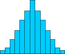
What if the data isn't symmetrically distributed, though? Consider the data set below.
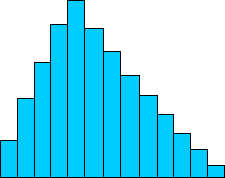
In this data set, the tallest peak is not at the center. If you calculated the average of this data set, you'd also find that the average doesn't correspond with the tallest peak. As a result, we must not only do our math carefully, we must also carefully select what kind of math we do so that we accurately represent the data. Having shown why an average is not always the best statistic to use when characterizing a data set, we can now turn to the definition and use of (this and) other measures of central tendency.
Mean (Average)
A mean (average) is perhaps the most well known measure of central tendency. In baseball, fans might talk about a pitcher's earned run average (ERA); students in a class might be interested in their grade point average (GPA). The average (also called the arithmetic mean--this is the typical sense when just the word mean is used) of a data set is the sum of all the data values divided by the total number of values in the set. Algebraically, a data set {x1, x2, x3,.,xN} has a mean μ defined as follows:
![]()
(Note that we use the Greek character μ, indicating that this is a population mean; the same formula applies when calculating the sample mean--you might see the sample mean expressed using ![]() in this case, for instance. The bar notation simply indicates a mean.) More generally, if we have a set of values {x1, x2, x3,., xN} with associated frequencies {f1, f2, f3,., fN} (recall how we defined a frequency in the previous lesson-here, we are simply saying that the data value xi occurs fi times in the data set), then we can define the mean μ as follows:
in this case, for instance. The bar notation simply indicates a mean.) More generally, if we have a set of values {x1, x2, x3,., xN} with associated frequencies {f1, f2, f3,., fN} (recall how we defined a frequency in the previous lesson-here, we are simply saying that the data value xi occurs fi times in the data set), then we can define the mean μ as follows:

The numerator of this expression simply says that the sum consists of each value multiplied by the number of times it occurs in the data set. The denominator is simply the total number of data values in the set (each value may occur more than once, so the denominator does not equal N).
A mean is best suited to cases where the data are symmetrically distributed, as with the first bar graph shown above. If the data is skewed, as with the second bar graph above, the mean is not as helpful. Consider the data tables below; the table on the left is a symmetrical distribution, like the first bar graph, and the table on the right is a skewed distribution, like the second bar graph. (You may want to try graphing these distributions to get a sense of how the tables and graphs relate.)
|
Data Value |
Frequency |
|
1 |
1 |
|
2 |
2 |
|
3 |
4 |
|
4 |
8 |
|
5 |
16 |
|
6 |
8 |
|
7 |
4 |
|
8 |
2 |
|
9 |
1 |
|
Data Value |
Frequency |
|
1 |
1 |
|
2 |
7 |
|
3 |
20 |
|
4 |
15 |
|
5 |
12 |
|
6 |
9 |
|
7 |
6 |
|
8 |
3 |
|
9 |
1 |
Table 2
Using the mean formula for data with associated frequencies, we calculate the mean of the data in Table 1 as 5. The mean for the data in Table 2 is 4.38. Obviously, the mean in the case of Table 1 does a good job of describing the data: the data value 5 is the most frequent value, and the other values show progressively lower frequencies. Thus, the mean shows the central tendency of the data set in this case. In the case of Table 2, the mean doesn't do such a good job: the most frequent value is 3, but the mean is between two less frequent values (4 and 5). As such, we must consider other measures of central tendency for non-symmetric data sets.
Practice Problem: Calculate the mean of the following data set:
{1, 2, 3, 4, 5, 7, 10, 15, 21, 22, 23, 24, 25, 26}
Solution: Simply use the formula for the mean μ as given above. The result is the same regardless of whether the data corresponds to a population or a sample. Note that this data set contains 14 data values.
![]()
![]()
Thus, the mean of the data set is about 13.4.
Mode
The mode is a measure of central tendency that corresponds to the most frequent data value. Referring once more to the example data tables above, the mode of the data in Table 1 is 5, and the mode of the data in Table 2 is 3. The mode always selects the "peak" of the frequency graph. In some cases, however, a data set may have more than one value that is the mode; this situation occurs when two or more values both have the same frequency and have the greatest frequency of any value in the set.
Practice Problem: What is the mode of the following data set?
{8, 1, 2, 0, 3, 6, 2, 8, 4, 5, 6, 1, 8, 6, 3, 9, 0, 9}
Solution: The mode is the data value (or values) that occurs most frequently. One way to find the mode is to draw a graph of the data (such as a histogram) and find the highest point on the graph. Alternatively, we can order the data set and look to see which value is the mode.
{0, 0, 1, 1, 2, 2, 3, 3, 4, 5, 6, 6, 6, 8, 8, 8, 9, 9}
By inspection, we can see that both 6 and 8 correspond to the mode of the data set. Note that if each value in a data set occurs the same number of times, the mode is not helpful.
Median
Another measure of central tendency is the median. The median is the value that corresponds to the middle of an ordered set of data; that is to say, exactly half the data values in a set are below the median and exactly half are above the median. The easiest (conceptually, anyhow) method of calculating the median of a data set is to write the data in ascending order, then find the middle value. If the data set has an odd number of values, the median is a clear single value; if the data set has an even number of values, there is no single middle value. Instead, in this latter case, the median can be defined as the mean of the two middle values. Thus, given an ordered data set {x1, x2, x3,., xN} with N members, we can write the median M algebraically as

The median is a useful measure of central tendency in cases where a few data values at one extreme or another have a disproportionate effect on the mean. Consider the data set below, which might correspond to the incomes (in thousands of dollars) of a certain group of people.
{24; 42; 64; 38; 49; 30; 34; 29; 2,350; 1,932, 61, 52, 51, 19, 28}
This set has 15 data values, so we do not need to calculate a mean of two middle values. To find the median, let's first rewrite the data set in ascending order. Next, we'll identify the middle value: this is the eighth data value, since there are seven values above it and seven values below it. The median is underlined in the ordered set below.
{19; 24; 28; 29; 30; 34; 38; 42; 49; 51; 52; 61; 64; 1,932; 2,350}
Let's now compare this result, 42, with the mean. Using the formula given above, we calculate the mean of this data set as approximately 320. Note carefully that the mean in this case is well above the incomes of the majority of the people from whom these data were taken--only 2 people in the group make at least the mean income, whereas 13 people (the vast majority) make far less than the mean income. The median income, however, does a much better job of expressing the central tendency of the data. If we were to ignore the two individuals with extremely high incomes, we would find the mean income of the remaining individuals to be about 40, which is close to the median income.
A slightly more difficult problem arises when the data values have associated frequencies; in such cases, writing a list of values may be quite difficult, since the number of values can be large. Nevertheless, the median can be identified without too much difficulty if an ordered list of values and associated frequencies is either available or is constructed. We know that in an ordered list of N values, the median is the value that falls in the middle. If the ordered list has associated frequencies, then the median is the value for which the cumulative frequency is N/2 (for even N) or (N + 1)/2 (for odd N). Of course, the index (N/2, for instance) of the median may not be equal to the cumulative frequency of a particular value; the index of the median, however, must be both less than the cumulative frequency of the median as well as greater than the cumulative frequency of the immediately preceding value. This concept is best illustrated by example, so consider the following practice problems.
Practice Problem: Find the median of the data set below.
{102, 403, 729, 843, 920, 360, 842, 941, 357, 483, 207, 670, 471, 109}
Solution: First, order the data. Note that because the set has 14 members, the median is the mean of two central values. These values are underlined in the ordered set below.
{102, 109, 207, 357, 360, 403, 471, 483, 670, 729, 842, 843, 920, 941}
Now, calculate the median M by finding the mean of 471 and 483.
![]()
The median of this data set is thus 477.


