
Set Up Data
Before you can practice with a pivot table, you need some data to use for the setup. Pivot tables answer questions, so your test data should be able to feed into the question. For instance, suppose that you have a list of products that sold each month. You could have a spreadsheet of a product sold by month. The following image shows some test data that we'll use with the rest of this article.
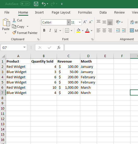
(Setup data for a pivot table)
In the image above, data is set up to list sales for two products: red widgets and blue widgets. The "Quantity Sold" column identifies the number of the respective widget sold. The "Revenue" column displays the revenue made from each widget, and the "Month" column lists the month the revenue and product were sold.
With a pivot table, you can answer several questions based on this data. The first set is to get the grand total of all revenue for product sold from January to March. After you get the grand total, you might want to know the revenue for each month. You can answer this second question with a pivot table.
Using the SUM Function to Get a Grand Total
You have a table that lists revenue for each month, but most spreadsheets run totals at the bottom of a column. The SUM function can be used to set up a total in the revenue column. You can also set up a total for the amount of widgets sold, but for simplicity we'll set up just a total revenue cell.
You should know that you have two options when entering a function into a cell. You can type the SUM function into the cell that you want to use for the total revenue, or you can use the function button next to the text input text box at the top of the spreadsheet. When you don't know parameters for a function, it's best to click the function button next to the input text box.
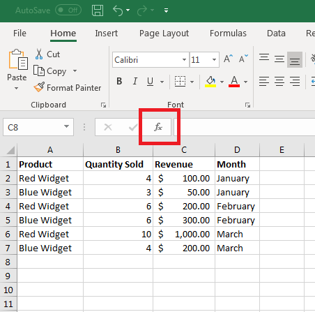
(Function button location)
Before you click the function button, select the cell where you want the total revenue to display. In this example, the cell that we want to use for the total amount is C8. Don't forget to add a label next to the cell to indicate to readers that the total amount is the total from the revenue column.
Click the "Function" button and the "Insert Function" window opens.
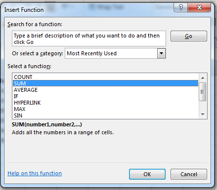
(Insert Function window)
With the "Insert Function" window opened, you can choose the function that you want to use. The SUM function is the second one shown in the image above, but you might need to search for it. Notice below the selected function is a description. The description includes the functions parameters and syntax. The description also displays a small explanation to help you identify what will happen when you include the function. The SUM function is self-explanatory, but you will need to read this description for some of the other more complicated ones.
Click "OK" and another window opens asking for you to highlight the cells that you want to add up. Highlight cells C2 to C7 and then press the "Enter" key. After you press the "Enter" key, a window displays showing the selected cells and a summarization of the results when the function executes.
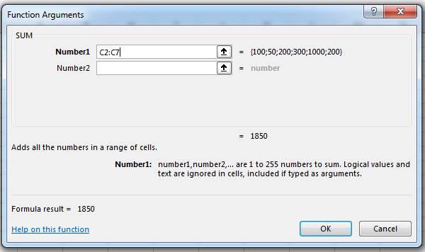
(Function arguments and SUM total summarization)
Notice that the bottom of the cell selected shows "= 1850" which is what will display when you click the "OK" button. Click the "OK" button and the total revenue now displays under the revenue entries. Because we formatted the columns as currency numbers, Excel 2019 automatically displays the currency character and decimal points.
Create a Pivot Table
Now that data is set up, it's time to insert a pivot table. The "Pivot Table" button is found in the "Insert" tab in the "Tables" category. Before you click this button, highlight all of the data including the total.
With the data selected, click the "Pivot Table" button. A new window opens with several options for the pivot table.
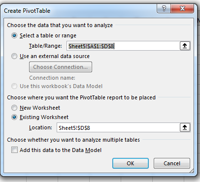
(Create Pivot Table window with settings options)
Notice that the Table/Range is already filled out, because we highlighted all of the data that we wanted in the pivot table before clicking the button. If we hadn't selected the data first, you would click the arrow button next to the input text box and select the data. After you selected the data, press the "Enter" key.
Notice also that you can choose an external source for your pivot table. Excel 2019 is compatible with several external sources that can store data. You can use a Microsoft Access database, which is also a part of the Office suite of applications. You can use another Excel spreadsheet file as a data source, or you can even use a high-end database such as SQL Server, which is an enterprise database solution also sold by Microsoft. SQL Server is often installed on an enterprise network where you need to store large amounts of data with millions of records. Microsoft Access is often found on small personal networks where data must be stored in a database but where SQL Server isn't necessary.
Another option for external data is an external database in the cloud. You need a connection on your computer, but then Excel 2019 can connect to this external connection which is then used to create a pivot table.
The second section of the "Create Pivot Table" window asks you where you want to display it. The default option is to display the pivot table in the same worksheet that you have opened with the pivot table's data. You also have the option to create the pivot table in a separate new worksheet. With this option, Excel will create a new worksheet and set up the pivot table in the new spreadsheet.
For simplicity, we will add the pivot table on the same worksheet as the current data table. The other option is where the pivot table should be located. Excel does its best to guess where you want to store your new pivot table, but you can click the arrow button next to the input box. This will open a new window where you can select the range of cells where you want to store the pivot table. Press "Enter" on the keyboard, and the new location for the pivot table is stored in the range for the pivot table location.
Since this is the default option, leave the settings as they are in the "Create Pivot Table" window and then click the "OK" button.
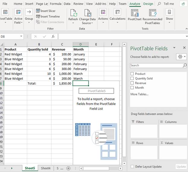
(Initial Pivot Table created with settings and column options)
The image above shows you what the initial pivot table looks like after you set up the data selection and location where you want to store it. The important part of the image above is the fields settings on the right of the pivot table location. The column names are shown in the fields on the right in the window with check boxes. These check boxes match the cells in bold at the top of each column. This is one reason it's important to always have labels with your data tables. Excel 2019 does its best to identify these labels and makes it easier to set configurations based on column or row names and headers rather than by standard labels. For instance, you can view column names in the configuration window as "Revenue" rather than C1 or the C column. With this example it's easier to identify columns without the custom headers, but when you have several columns or rows with different labels, it can get confusing especially for an outside viewer that has to work with your data table.
In our original question, we wanted to know the amount of revenue for each month. Check the "Revenue" and "Month" check boxes in the right column to add them to the pivot table. An even better way to answer this question is to identify the amount of revenue per month for each widget product. For this example, we'll check the "Product" check box as well. The pivot table now displays with answers to the data question asked from the pivot table.
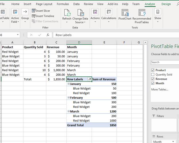
(Pivot table showing revenue by product and by month)
Notice that Excel 2019 automatically groups columns and data using the column labels that you chose in the window to the right. With a pivot table, you can easily change questions and get an answer to these questions. For instance, suppose you no longer want to get revenue by product, but instead you want to just see revenue by month. By removing the check mark next to the "Product" label, you remove the product column from the pivot table's calculation and show an answer to the question "How much revenue was made by month."
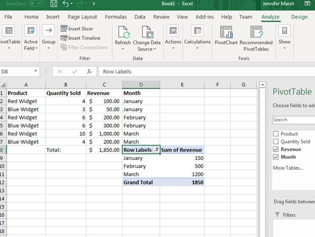
(Pivot table display revenue by month)
With a pivot table, you can add and remove columns in your calculation as needed. You can also add additional pivot tables to your spreadsheet should you decide to add another one based on a subset of data. Just like charts and graphs, Excel 2019 lets you create several pivot tables using one set of data but using a subset of this data.
Pivot tables are beneficial when you need several output results based on the same amount of data. They are the table version of a chart, which can also be used to provide a visual representation of your data. With a pivot table, instead of showing data for just one answer to a question, you can have several different options that answer several questions with just a few clicks of the mouse.