The VLOOKUP Function

It's important to remember that lookup functions require two columns (or rows when using HLOOKUP). The first column is searched for a given value, and then the adjacent cell to the right of the column is the data used to either calculate a result or just display the lookup result in the spreadsheet. These lookup functions make it easier to find values among hundreds (even thousands) of records in a spreadsheet instead of searching for a value using a simple file search. They also provide a way to perform a lookup and display data dynamically should the value in the lookup column change.

The VLOOKUP function uses the following syntax:

VLOOKUP (<data to search for>, <cell range to search>, <the column number in the cell range to return after a match>, [OPTIONAL]<return only an exact match>)

The result from a VLOOKUP can be used in an additional calculation, or you can simply display the result in the selected cell. VLOOKUP only uses columns to search for data, so any values used in the function's parameters will base a search on columns not rows.

(VLOOKUP function example)

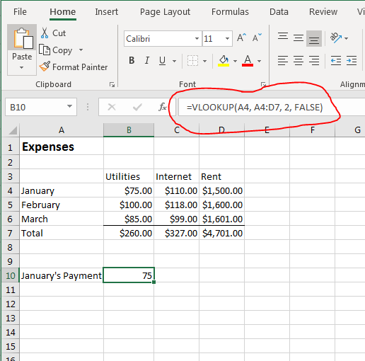
Using the "Expenses" spreadsheet, you can use VLOOKUP to find a value in any month's record. This spreadsheet only has a few records but imagine having a spreadsheet with several years of data. Scrolling through all records could be time-consuming, and you could miss values by just doing a quick review. The VLOOKUP function can be used to highlight all records and perform an automatic lookup.

In this example, VLOOKUP searches all records for the "January" string. This example uses the A4 cell reference, but you can also use "January" in the first parameter instead. Static values are usually frowned upon, because changes to the cell are not dynamic with other functions n the spreadsheet. The second parameter specifies the range of cells to search. The third parameter tells Excel which adjacent cell in the row to use. The second column is the "Utilities" field, so the VLOOKUP function retrieves the $75.00 payment from the lookup. For instance, if you entered "3" for the third parameter, the VLOOKUP function would return the "Internet" column payment of $110.00.

Excel lookup functions provide a way to return values that approximately match a search. If you want this type of search, you would use "true" in the optional fourth parameter. The issue with approximate searches is that you don't get a precise return value. Similar searches should be used with care to avoid errors in your calculations, so it's best to use the "false" option as the fourth parameter.

The HLOOKUP Function

VLOOKUP performs searches based on columns, but the HLOOKUP function gives the opposite type of search using rows. The parameters and syntax for HLOOKUP are the same, except instead of specifying the column from the left side of the selected cell range, you use parameter values that specify the row cell that you want to return from the top of the search range.

(HLOOKUP function example)

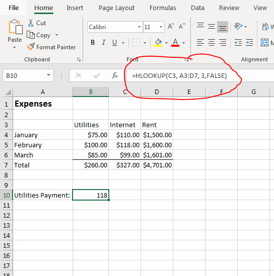
For this example, the same range of cells is used to search for the "Internet" payment for February. You aren't limited to the first row after the main lookup row, so this example shows you that you can return the value several rows below the main header row.

Instead of basing a search on columns, this HLOOKUP performs a search on payment records for each type. The C3 cell contains the value "Internet," so the lookup finds the cell with a value of "Internet," and then it returns the value in the Internet column that is three rows down from C3 (including C3 that Excel 2019 allocates as row one). In this example, the value in the "Internet" column three rows from the C3 (including the C3 row) cell is $118.00.

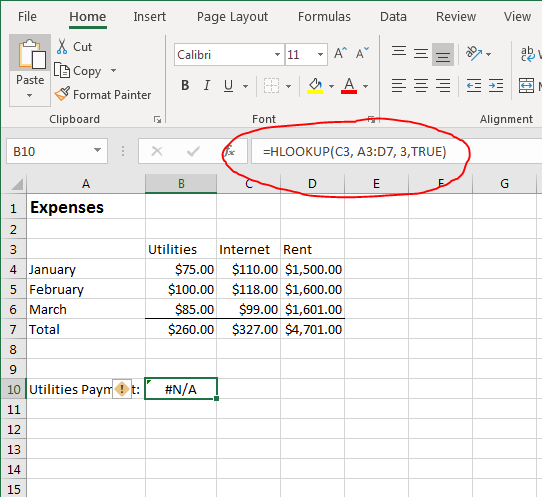
The last two examples used a "false" value for the optional "Exact Match" parameter. This will be common for most lookups, but you can also work with an approximate match. This will find a value that best fits the search parameters. The one requirement for this type of search is that your data must be in ascending order. For this reason, you can only use an approximate match lookup when you have data that you can sort. Spreadsheets such as the example "Expense" report would not be able to work with an approximate match lookup, because you cannot order data.

If you attempt to perform a lookup using an approximate match with data that is not in ascending order, Excel returns an #N/A error.

(HLOOKUP using an approximate search without ascending data)

If you see "#N/A" shown in a cell with either a VLOOKUP or an HLOOKUP, you know that you must switch the approximate search to an exact match by changing the parameter to "false."

The LOOKUP Function

VLOOKUP and HLOOKUP functions have been a part of Microsoft Excel's internal functions for years. In later versions, Microsoft introduced the LOOKUP function, which gives you greater control of the way that you search for data. VLOOKUP only works with vertical searches. HLOOKUP only works with horizontal searches, but the LOOKUP function lets you perform a search both vertically and horizontally.

The LOOKUP function works similarly but has different requirements and results. Microsoft suggests that users should use the LOOKUP function when you only need to only search one row. This method is called the vector form, and the result displays the first value found in the row or column. The array form lets you search additional columns and rows, but the search feature is much more limited. Microsoft recommends sticking to the two alternative VLOOKUP and HLOOKUP functions when you need to search multiple columns and rows.

The syntax for the LOOKUP function is as follows:

LOOKUP(<value to search for>, <cell range to search>, <cell range to retrieve a result>)

•          Value to search for: the value that you want to find in a range of cells.
•          Cell range to search: the range of cells that should contain the search value.
•          Cell range to retrieve a result: values to retrieve when the lookup detects a matched search value.

  Notice that the LOOKUP function does not have an approximate or exact match option. The first three parameters are similar to VLOOKUP and HLOOKUP, but the ranges must be the same or LOOKUP will return an error. LOOKUP is best when you have a simple number of search cells and you just need a simple result from a group of values.

   

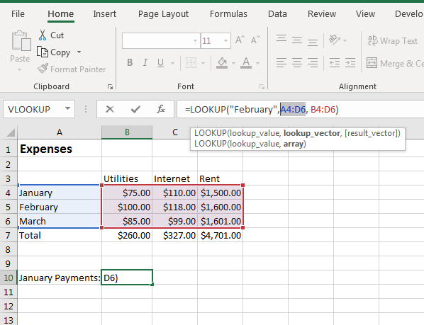
  (LOOKUP function example for a row)

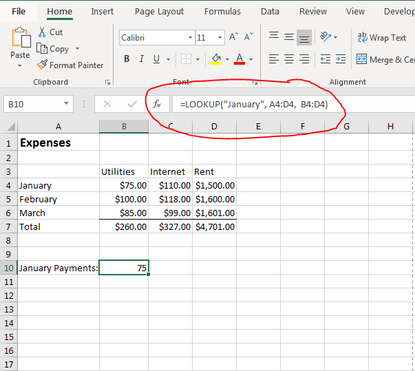
  The first "January" row is in ascending order, so you can quickly find the first value that matches the "January" search term. Notice that Excel returns the first value that it finds adjacent to the "January" text. LOOKUP will work with numbers, text or logical values, so you aren't limited to just numbers. However, text searches are better for VLOOKUP and HLOOKUP for the approximate search option.

  With the LOOKUP function, the search range and the range to retrieve should be a similar size. If you perform a search with an incorrect range to retrieve values, Excel returns an #N/A error.

  

  (LOOKUP function #N/A error due to selected range)

  Because it's easy to trigger an #N/A function error, you should work with only one row or one column with the LOOKUP. The "January" LOOKUP function example found the term "January" in the row of values. You can easily find these values by doing a quick review, but you could have thousands of cells in a row or column, so this example is useful when you want to find the first result in a row.

  LOOKUP can be used for columns as well. You might want to know the first payment made in the "Rent" column. You can use the LOOKUP function to search the column for results in this column rather than in a row. This can be useful to identify values in a specific column rather than a range of cells.

  

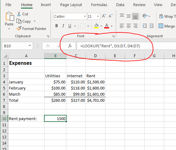
  (LOOKUP function column example)

  Again, the LOOKUP function detects the first value it finds in the selected cells and displays it in the function cell. The column lookup feature is similar to searching a row where if you select a range that's too small or too large compared to the search cells, you can trigger an #N/A error.

  The LOOKUP function also lets you simply specify if the search term is found. You can perform a simple search by eliminating the third parameter. By eliminating the third parameter, Excel 2019 returns the search phrase itself if it's found during the lookup.

  

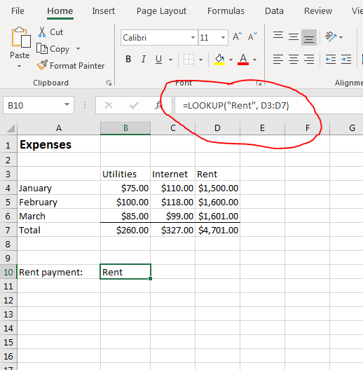
  (Simple LOOKUP with no result cell range)

  When you don't specify the result that you want to display, Excel 2019 uses the default search term. When you search for "Rent" within a range, "Rent" is returned to the selected cell. Using the LOOKUP function in this way creates a simple search that shows you if a search term does indeed exist in a selected range.

  Data lookups are common in complex spreadsheets that have thousands of data points. You can't eye values without scrolling through every record, so using a lookup function makes it easier to reference values with just a few clicks of a mouse. Data contained in cells will dynamically recalculate should the information change, so using data lookups makes your spreadsheets much more functional when you have data that changes frequently.