
Basics of Pivot Tables
Before you create a table, you should understand the difference between a pivot table and creating a basic chart. A pivot table is meant to take a long list of data and summarize the results. With a standard chart, you must reorganize data so that you can change the way a graph displays data the way you need it to. With a pivot table, you can "pivot" your data so that you can summarize and review it with a different data set.
The other difference between a pivot table and a standard chart is that pivot tables are more interactive. Both pivot tables and charts will update data dynamically, but you can dynamically change the summary data in a pivot table while charts only change data changed in referenced cells. You can change the way a table is displayed with just a few clicks of your mouse with a pivot table, so it's mainly used as a way to quickly review information and get a high overview of what information a worksheet contains.
Pivot tables can be created on complex or simple data, but they are usually beneficial when you have a long list of unorganized records that don't have any sort or normalization set. You can pull records from a database, a CSV file, a JSON file, an XML file, Access or any entity that has structure so Excel 2019 can determine the rows and columns used to summarize data. Structured data is common in many databases but pulling data from a source such as a web page will not have the same structure that can be used for pivot tables. Some web pages provide structured data, but in many cases, you'll need to clean up data if you pull it from a web page and want to use it for pivot table analysis.
Although you might use pivot tables to analyze data, you can still add charts and graphs later. Excel 2019 includes a feature that lets you link a pivot chart to a pivot table, so you can both analyze data using the information summarized in a pivot chart and then display the results using a pivot chart for visual representation.
Creating a Quick Pivot Table
You can import data directly from a database and create a pivot table using Excel's import tool. Using a sample SQL Server database that contains arbitrary data about titles, genres, payments and customer information, a pivot table can be used to determine payment amounts from members. Using a pivot table, you can determine membership payments for each day of the month. Pivot tables are typically used when you have a long list of data where only certain columns distinguish the information that you need from it.
For this example, a table of membership payments was imported from a SQL Server table. You can import data by clicking the "Data" tab and then clicking the "Get Data" button. In the dropdown, select "From Database" and then click "From SQL Server Database" in the submenu. Follow the prompts to configure the SQL Server database that you want to connect to and at the last import step, you can see the option to import to a new pivot table.
(Pivot Table import using "Get Data" tool)
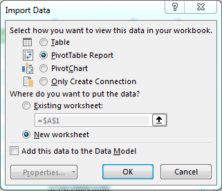
Using Excel's import tool, you can automatically create a pivot table without performing any additional steps. This is the easiest way to create a pivot table when you have data from an external source and don't know how to create one. Click "OK" to create a pivot table and create it in a new worksheet.
After you decide to import to a pivot table, Excel 2019 opens a configuration window to help you determine the data that you want to use.
(Pivot Table configuration)
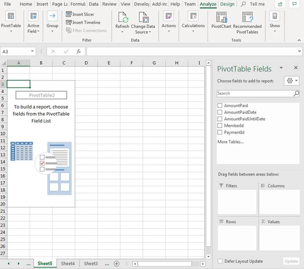
Excel needs to know what fields that you want to use in your table. In the "PivotTable Fields" section of the configuration panel, choose the fields (columns) that you want to analyze. In this sample, customer payments will be analyzed to determine how much money was made each day in the month of February. With this goal, we need the "AmountPaid," "AmountPaidDate," and "MemberId." Check these boxes and notice that Excel automatically transfers column data to the active worksheet.
(Pivot table created)
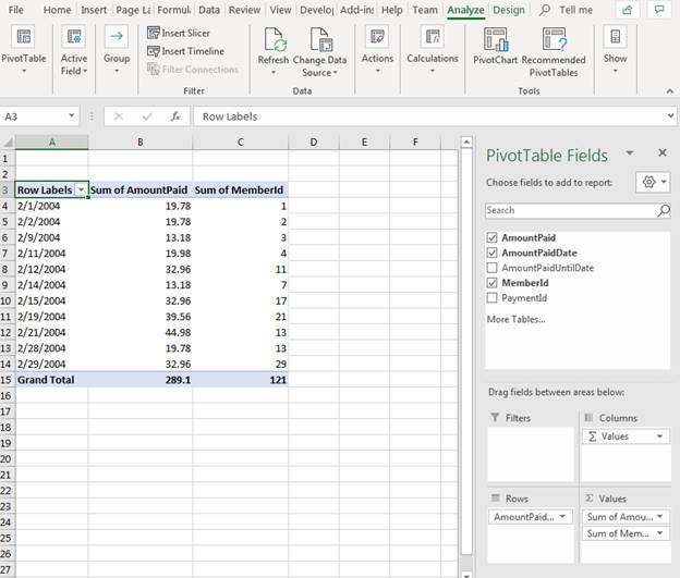
Pivot tables group your information into understandable summaries. You don't need to write complex SQL statements to create a data set that summarizes data when you have pivot table creation procedures in Excel 2019. Notice in the new pivot table that data is summarized by day of the month. The total amount of revenue for each day is automatically summed and displayed per day.
In this example, the member ID was included, but after reviewing the spreadsheet you can see that member ID is not necessary. The pivot table summarizes the member ID as if it's an integer, so it doesn't fit with the other data set. Instead of manipulating data and re-organizing it, you can remove this column by unchecking the "MemberId" column in the "Pivot Table Fields" configuration panel.
(Edited pivot table)
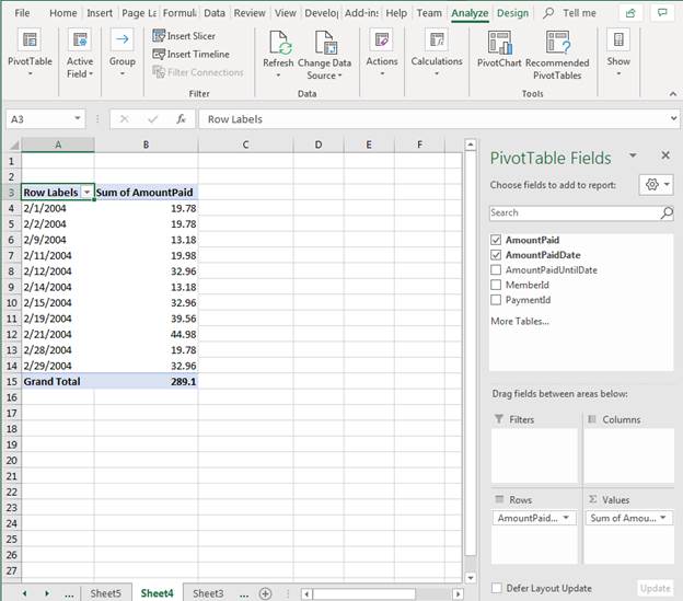
By unchecking the column in the "Pivot Table Fields" configuration panel, the member ID is immediately removed from the worksheet. With just a click of your mouse, you can change the way your pivot table displays data.
Editing Summarization Functions
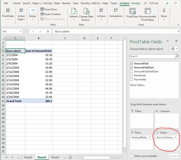
When you create a pivot table, the default function used for data aggregation summarization is SUM. The SUM function simply adds values and displays a total. The "AmountPaid" field was detected as a decimal value and automatically summed when you created the pivot table, but you can choose to perform other mathematical functions on table data. The "Pivot Table Fields" configuration panel has a section where you can change the function used.
(Function settings option)
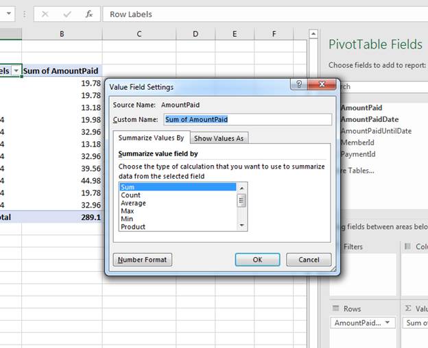
Click the dropdown and select "Function Field Settings." A window opens where you can configure the function used in the summarization cell.
(Summarization function selection settings)
The "Custom Name" text box is where you set the column header. Excel 2019 automatically sets it as "Sum of <field name>" where "field name" is the name of the column configured in the database. You can change this to a column header value of your choice.
In the second section of the settings window, the "Summarize value field by" list shows you the internal Excel functions that you can use to summarize data. Notice that you can use Count, Average, Min, Max, Product and numerous others. For instance, change the function used to Count and Excel will count the number of payments instead of summing values.
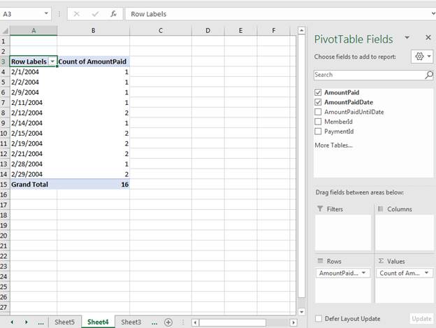
(SUM function changed to COUNT)
With the SUM function changed to COUNT, notice that now the summarized field displays the number of payments. The COUNT function is also used to count the number of payments for each day instead of summing the values for each day. This easy change of data and the way it's displayed is the advantage of using a pivot table rather than manually laying out spreadsheet data and reorganizing it every time you want a new chart.
Editing "Group By" Field
Because the goal of the first pivot table was to identify the amount of revenue per day, Excel groups payments by day of the month. Remember that the advantage of pivot tables is to quickly change the information displayed in a table. Suppose you want to view the amount of revenue per customer for the month of February. You can change the pivot table to display this information instead with a few clicks of the mouse.
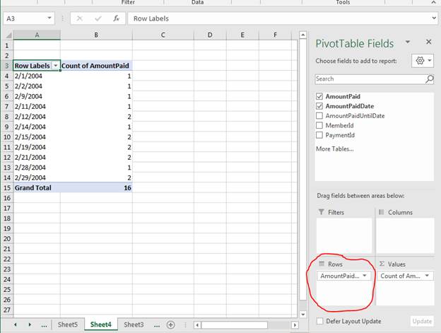
To change the field used to group data, you change the value in the "Rows" setting.
(Row function changes)
Before you change this setting, you must add the table fields relevant to your search. Since the new table will show payments by customer, you need the "MemberId" field and the "AmountPaidDate" field. Uncheck the unnecessary data and then check the box next to these two fields in the configuration panel.
When you first change the field columns, Excel again attempts to detect the right functions to use and the way that you want to summarize information.
(Incorrect summing values)
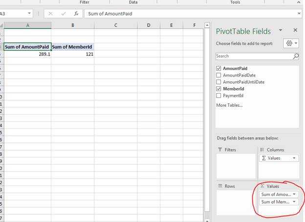
With the new data incorporated into the pivot table, Excel things that you want to sum the amount paid and the member IDs. This isn't correct, so the pivot table needs to be configured to display a sum of payments based on customer. In the "Values" section, click the dropdown arrow and choose "Remove Field" for each field. This resets the pivot table to a blank placeholder.
You can now specify the "group by" column and the column that must be summarized. Excel provides a drag-and-drop feature for pivot tables where you can specify the columns for the "Rows" (group by) section and the columns for the "Values" (summarize) section. Drag and drop the MemberId column to the "Rows" section. Then, drag and drop the AmountPaid column to the "Values" section. Now, you can see that Excel knows what to do with the data you've specified.
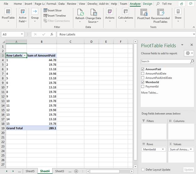
(Corrected pivot table)
With a combination of row and value settings, you can determine the way data is presented in a pivot table. It might take a few changes before you get the information that you need, but just remember that the rows determine how data is grouped, and the values section determines the functions to summarize data.
Adding Filters
In some scenarios, you want to filter out some data. Or display only certain values. You can do this by dragging and dropping an additional column in the "Filters" section. For instance, you might only want to see a value for a specific payment ID. By dragging and dropping the "PaymentId" column to the "Filters" section, you can add a filter option to the top of your pivot table that can be used to control the data displayed.
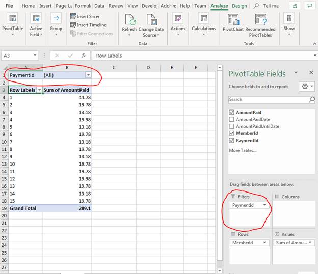
(PaymentId filter added)
With the PaymentId added to the "Filter" section, Excel adds it to the top of the spreadsheet. You'll see that the default filter selected is "All," which means all data is shown. Click the dropdown arrow to see a list of payment IDs included in your data. Although you can't see payment IDs in your pivot table, it's still a part of the imported information from the database. You can still filter on a column that isn't included in the data that displays in the table, because it's a part of the included fields listed in the configuration panel.
Click any payment ID in the dropdown list, and Excel eliminates all data except for the selected ID.
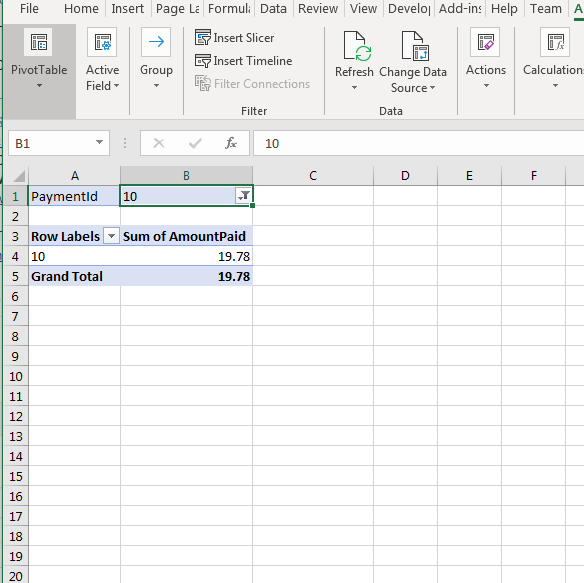
(Filtered data by PaymentId)
The pivot table eliminates all other data and displays the total amount in the payment ID of 10. You can use a filter with any column including ones that are already displayed in your pivot table. If you choose to have multiple filter values, click the dropdown again and check the box labeled "Select multiple items." Select your filter and click "OK."
These basic pivot table features get you started for more advanced tables that incorporate multiple tables and data points, which can be imported and used in several spreadsheets, databases, files or any external source that works natively with an Excel connector. You can still chart and graph your results with visual representation, but pivot tables are the first step towards dissecting information and presenting it in a way that gives you answers to your questions.
Create a Calculated Field
Pivot tables summarize data stored in a worksheet to provide information about your data. You might have additional calculations that aren't a part of your data but it's a calculation that you need to get a bigger picture. For instance, with membership fees there could be a cost to process the payment. Even though you can see revenue for each day, you must add costs into the equation so that you can see total revenue. You can display the fee in a separate column or simply subtract a percentage to see net revenue rather than gross.
Since a pivot table only displays data directly from a source, you won't have this information available as a configurable column. You can, however, create a calculated field that takes the data from a pivot table field and calculates a result. It's similar to adding a formula to a cell except it uses pivot table data.
Click the pivot table field that you want to use as a part of your calculation. If the "Pivot Table" menu is not active, click the "Pivot Table" menu option in the Excel quickbar. The "Analyze" menu activates, and you can find the buttons to create a calculated field in the "Calculations" section of the menu.
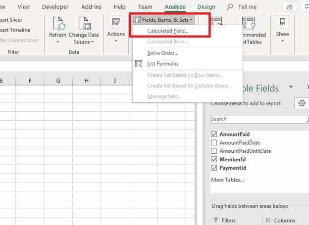
(Fields, Items, and Sets dropdown to add a calculated field)
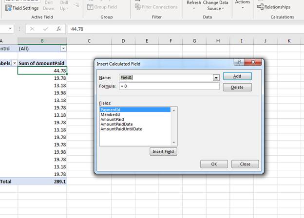
Click "Calculated Field" and a window opens that asks you to enter the formula for your calculation. The "Insert Calculated Field" window lets you configure a new column that will also be a part of the pivot table even though the data is not a part of the source.
(Insert Calculated Field window)
The "Name" field is the name of the column that will display in the pivot table. The "Formula" is the calculation that you want to use in the column. The "Fields" list displays the available fields that you can use in your calculation. Instead of typing the field name, you can select the field and click "Insert Field." Excel then adds the field name to the calculation.
(Added calculated field)
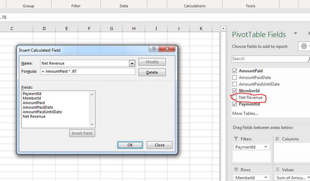
After creating a formula, click the "Add" button and Excel adds the new column to the list of available fields in the right pivot table panel. You can also modify the field by clicking it in the list of fields and modifying the formula. When you are finished, click the "OK" button.
Since the new calculated field is added but not activated, check it in the list of pivot table fields to add it to the worksheet pivot table. With a calculated field, you can now view additional information that isn't in the table but need to know about your data to get a full picture.
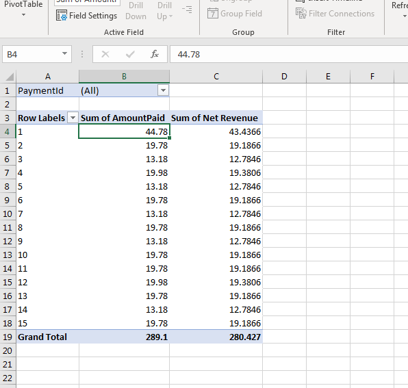
(Pivot table with calculated field)
The example table does not have currency formatting, but you can see the net revenue based on the formula. The formula subtracts 3% from the "Amount Paid" column and displays the net revenue in the "Sum of Net Revenue" column. Because the data in a pivot table is a summary of each day's revenue, the "Net Revenue" column is also a summed value.
Calculated fields are beneficial when you need to add columns for data that does not exist in the main data source. Instead of manually calculating additional information, calculated fields display the additional information that you need.
Adding More Complex Calculated Fields
The previous section used a simple formula to calculate a percentage to display a column with net revenue. You can incorporate Excel functions with your pivot tables and calculated fields. Using a function with your calculated fields is the same process as adding a function in a standard worksheet field.
Suppose that you have a sliding scale fee for payments. You might pay 3% on charges under $5 but 4% on transactions over $5. The IF function can be added to your calculated field to make a specific calculation based on the value of each pivot table row.
Click the "Fields, Items, & Sets" button in the "Calculations" section of the "Analyze" tab, and then click "Calculated Field" menu option to open the configuration window. All other configurations are the same as a simple calculated field, but now you add the IF function to the formula.
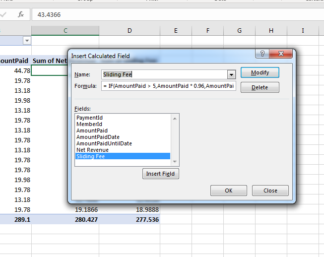
(Calculated field with the IF function)
With the IF statement, the calculated field is multiplied by .97 if the pivot table value is lower or equal to 5 and multiplied by .96 if the value is greater than 5. This calculated field gives you the ability to quickly sum revenue values based on input without manually calculating net revenue. Calculated fields aren't limited to just one function. You can embed functions, add additional formulas to your field and use any Excel function that you can use in a standard worksheet cell.
Should you ever want to remove or modify your calculated field, click the same button and menu option to open the configuration window. If you delete the calculated field from this configuration window, it's immediately removed from the pivot table. You can also modify the formula and change the way a calculated field works in this window.
Using Slicers
The field configuration panel has a filters section that you can use to control the way data displays in your pivot table, but Excel has a more powerful tool for filtering data called a "slicer." A slicer lets you take data already in the pivot table and create a button panel for quick filtering of your data.
The "Filter" section of the pivot table main menu has a button labeled "Insert Slicer" used to create a slicer in your spreadsheet.
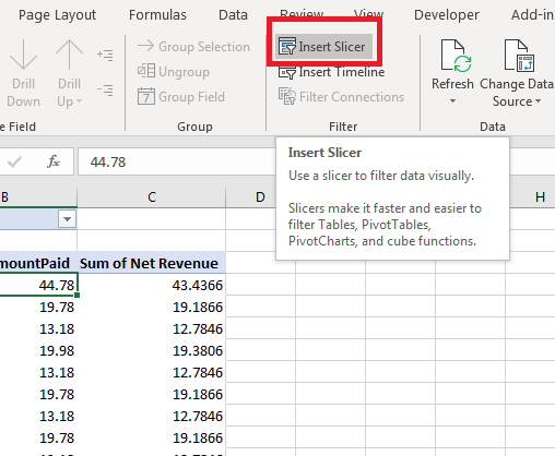
(Insert Slicer button)
Click the "Insert Slicer" button to open a configuration window. This configuration window simply displays the columns that you want to use in your filters.
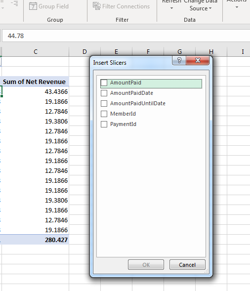
(Insert Slicers configuration window)
Check the box next to at least one column. The data in the column is used for the filter, so you would only use slicers on specific columns that have limited but unique data. In this example, the pivot table displays payments for each day of a month. You can use the "AmountPaidDate" column to filter payments by each day to get a summary of the payments for any selected day. PaymentId would be a poor choice for a slicer, because each payment has a unique ID. If you had 1000 payments in a table, a slicer would have 1000 filter options, and each filter would only have one result.
For this example, the AmountPaidDate column is chosen. Click "OK" and the slicer displays in the worksheet. You can click any one of the slicer choices, and the pivot table is automatically filtered using the selected slicer value.
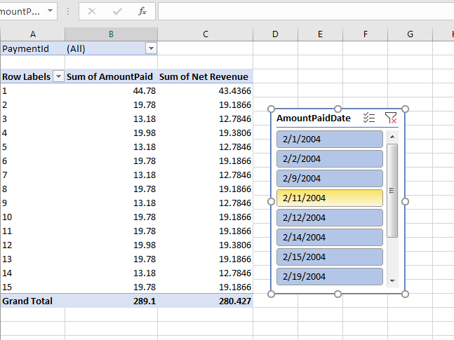
(Slicer added)
In this example, each day of the month of February is shown as a slicer option. Notice that not every day of the month displays, because a slicer only takes the data logged in the table. Since no payment was logged in 2/3/2004, this date is not shown in the slicer. Clicking any one of these slicer options will filter data to display only payments from the selected dates.
Use slicers when you want a GUI with better functionality than the standard pivot table filter option. Slicers make your pivot table more easily functional, meaning should you distribute your Excel spreadsheet to other users, they can easily understand that clicking any one of these filters will limit data to the selected value.
Hiding and Showing Subtotals and Totals
When working with large tables with several subtotal and total rows, you might want to remove these rows to reduce the amount of space needed to display the pivot table information. These options can be found in the "Layout" section of the "Design" tab for your pivot table.
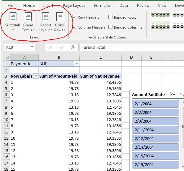
(Layout options)
Click one of the buttons in the "Layout" section and view the options. For instance, the "Subtotals" button displays a dropdown with a list of options on how to display this value.
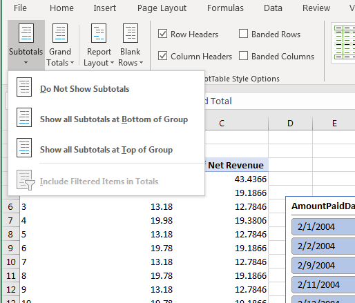
(Subtotal options)
You can choose "Do Not Show Subtotals" to hide them from your pivot table. You can also choose to place them at the bottom or top of the pivot table. The same can be done with grand totals by clicking the "Grand Totals" button.
The other two options in the "Layouts" section is the report layout and how to deal with blank rows. The "Report Layout" button will let you use preset designs available in Excel. The "Blank Rows" button gives you the option to add a blank row after each line item or remove any blank rows after pivot table line items.
Adding a Timeline
Not all data is based on numeric values. Some pivot table values are dates and text. It's not uncommon to get a snapshot of your data based on dates, but you need more than just a filter that displays individual day values. Excel 2019 has a feature called a timeline that lets you create a different type of filter based on date ranges. Timelines have a similar function as a slicer, except instead of using values in a row, you use date ranges for columns that contain date values.
The timeline feature is found in the same section of the menu as slicer button. The "Filter" section of the "Analyze" menu has the "Insert Timeline" button. Click it to open the timeline configuration window.
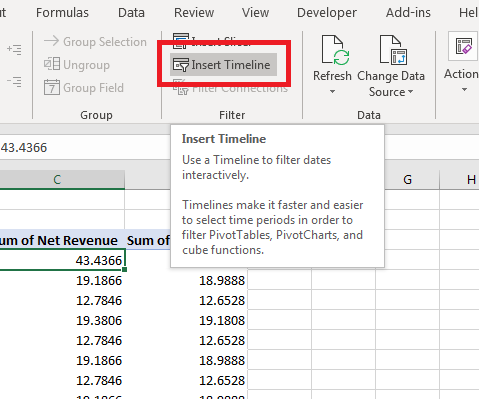
(Insert timeline button)
The slicer configuration window displays all columns in the pivot table, but Excel detects columns that contain dates and filters out all other fields.
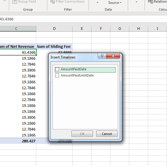
(Insert timeline window)
Check the columns that you want to include in your timeline. In this example, the AmountPaidDate column will be used to filter records based on the day that a customer paid a membership fee. Click "OK" after you make your column selection. A timeline filter is then added to your pivot table worksheet.
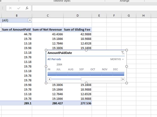
(Timeline filter)
An Excel timeline shows a clickable button for each month. Because the dates in the AmountPaidDate column are set to 2004, the year is automatically set to 2004. If you have multiple years, they will display in your timeline. Click one of the months in the timeline and Excel filters data to display only the currently selected month. The sample data in this pivot table only has the month of February stored, so only the "Feb" filter will display any data. However, if this was a long list of payments across several months, you can click each month to see only the selected month's data.
Use timelines when you have several rows of data but need to see a snapshot of just specific dates. Instead of limiting the imported data, working with timelines lets you import all records and then filter based on your own configurations.
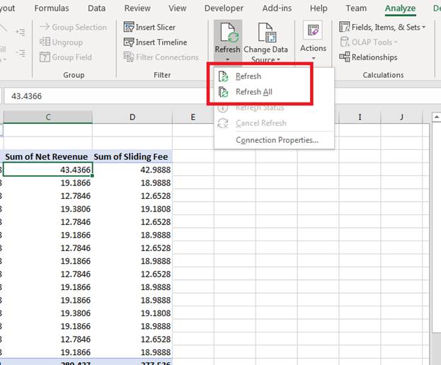
Refreshing Data
Pivot tables that have live, dynamic data behind them need a data refresh regularly. Your data from today might be different tomorrow. Outdated data skews your numbers and gives inaccurate report information. Since you already created your pivot table, recreating it after importing the table again would be time consuming. You can refresh your data at any time after you've created a pivot table to preserve your configurations but update data to the latest information.
(Refresh data options)
The "Data" section of the "Analyze" menu has buttons for refreshing data and changing the data source. Changing the data source will alter the entire structure of your pivot table, so only use this feature if you need to change the information shown in a pivot table.
Assuming that you don't need to change the connection properties, click "Refresh" to update the data. If you have multiple pivot tables, you can refresh all data across every worksheet by clicking the "Refresh All" option.
Excel offers numerous pivot table features so that you can "pivot" information and get snapshots of several data points. Use these tables on data stored in a database, file or other resource to get a better overview of the way your information tells a story of important parts of your business.