Location of Image and Graph Functions
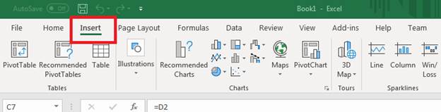
You should notice that the "Home" and "Data" tabs contained all of the functionality needed to format text and insert What-If Analysis tables. The "Insert" tab has several functions for adding objects into spreadsheets including images.
(Insert tab)
Click the "Insert" tab and take a look at the buttons included within this tab. It contains several options to insert a pivot table, a standard table, illustrations, charts, maps, and shapes. The "Illustrations" button contains a dropdown menu that includes the option to add images. This chapter covers images, icons and shapes included in the "Illustrations" button dropdown options. Note that the "Illustrations" button shows as a dropdown when Excel is sized to a smaller window. If you expand the working Excel window, "Illustrations" is shown as a category of options in the "Insert" tab.
Adding Pictures
The first option from the Illustrations dropdown is the function to add pictures.
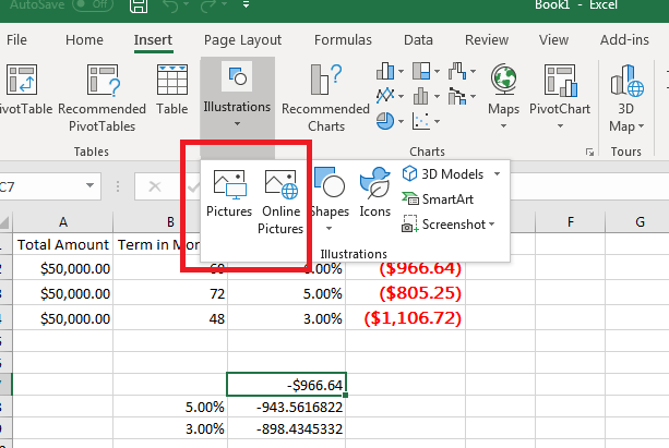
(Pictures and Online Pictures option in the Illustrations dropdown)
The "Pictures" selection lets you add a picture from your local storage drive. First, click a cell anywhere on a current worksheet. Next, click "Pictures" and an "Open File" window is opened. Select an image stored on your local hard drive and then click "Insert." An image is added to the currently active selected cell.
Images found online provide much more variety, so if you don't have your own images but need to find one for your spreadsheet, Microsoft has a collection online where you can choose an image from a variety of categories on Bing. Bing is Microsoft's search engine, and it has been integrated into some functions in current versions of Microsoft Office including Excel.
Click the "Illustrations" button again, and then click "Online Pictures." A window opens with several categories shown.
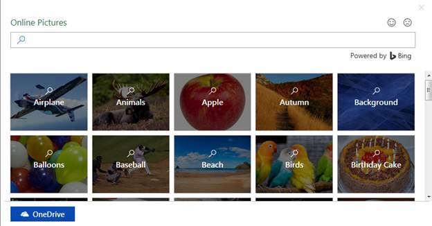
(Online picture categories offered by Microsoft)
You can search these images or scroll through the list to choose an image. For instance, click the "Apple" image. A new window opens where several types of apple images display. Cartoon images, sketches, snapshots of apples, and even the old Apple logo is displayed. You can use any of these images in your personal spreadsheets, and Microsoft adds them to it from their online collection. Notice that images are from an online collection using Bing. Using this tool saves time, because you don't need to search Bing and filter through several unrelated pictures.
To add the image to your spreadsheet, click one of the apples and then click the "Insert" button. You can add multiple images from the online collection by clicking each one individually and then clicking the "Insert" button.
Notice that the image is added to the spreadsheet in the currently active cell. Microsoft fits the image into the spreadsheet but uses the size from the original image. Click the image to make it the active object in the spreadsheet. The line surrounding the image has several circles located on the sides and corners of the object. These circles indicate locations where you can change the size of the image to better fit the spreadsheet size.
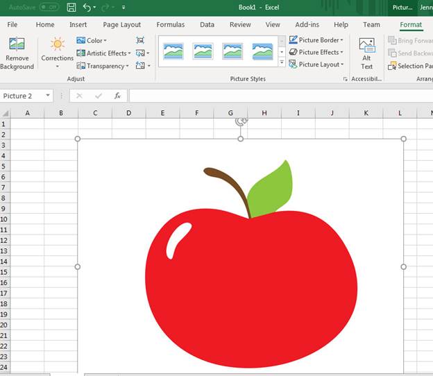
(An inserted image in a blank worksheet)
Click the bottom-right corner circle (not shown in the image above) and resize the image to fit a smaller screen width. Using the corner circles, you ensure that the height and width of the image are resized evenly. The circles on each size will only make the image width or height smaller, so the image's quality is compromised.
The arrow at the top of the image can be used to rotate it. Suppose that you want to display the apple laying on its left side. Click the arrow at the top and move the mouse left and right until the image is displayed the way you want.
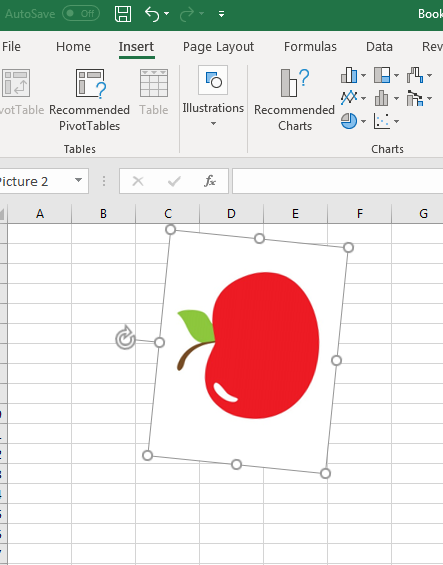
(An image resized and rotated to the left)
If you change your mind and want a different picture in your spreadsheet, right-click the apple (or the image that you chose from the online list) and click "Change Picture." In the submenu, choose where the new image is located. You can change a picture to one that is stored on your hard drive, or you can choose a new picture from Microsoft's online collection.
Excel has several pre-designed filters that you can use to change the look and feel of your added picture. Right-click the image and select "Format Picture." A window displays next to the image with several options.
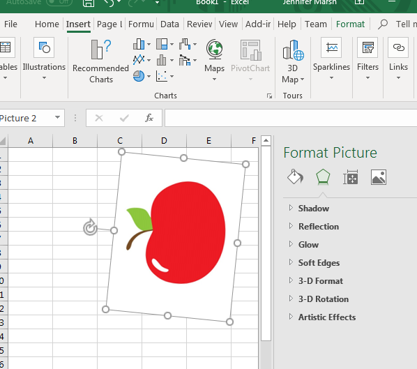
(Excel's list of filters to enhance an image's look and feel)
For instance, suppose that you want to add a drop-shadow to an image to enhance the way it displays on the spreadsheet. Click the down-arrow next to the "Shadow" menu item and then click the "Presets" button. Several drop-shadow options display the way an image will look after you add the filter. Choose one of them and the effect is added to the image.
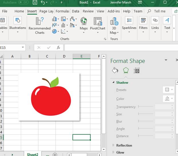
(A drop-shadow added to a spreadsheet image)
These filter effects add a special look to an image without the need to ever use specialized graphics programs. Remember that if you ever add a filter effect that you don't like, you can click the "Undo" button to reverse the effects.
Click the image and notice that a new "Format" tab item displays. Click this tab, and you see several other effects that can be added to an image. You can adjust the image's transparency, color and artistic effects. After you've added an image, scroll through these artistic effects to see what they do to an image's look and feel.
The "Picture Styles" adds outline formatting and image changes such as turning a square image into a circle. Excel has several picture styles to choose from, but it shows a sample of what the image would look like should you apply the effect. This will help you choose a style that best works for you.
Adding Shapes
For spreadsheets with workflows, you need a way to add shapes. Excel has numerous shapes to choose from, so you don't need to create triangles, squares, arrows, circles and any other preset shape that you can think of. You can add a shape by clicking the "Shapes" button from the "Illustrations" dropdown.
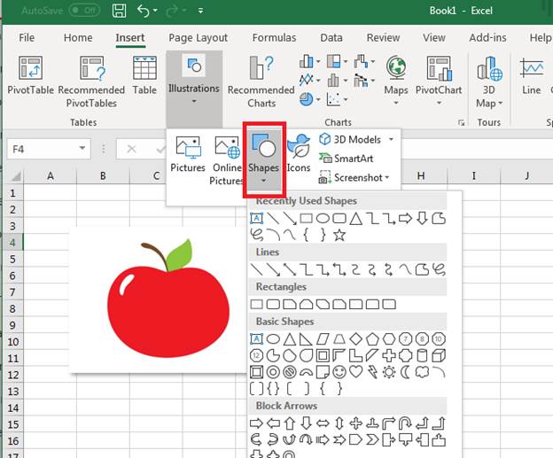
(Adding shapes)
When the "Shapes" button is clicked, several are shown in an additional dropdown. The image above shows only some of the shapes available, but you have several more that you can scroll through. Adding a shape requires the same steps as adding a picture, except Excel prompts you to assign a size to the shape.
Click the shape that you want to add, and Excel returns to the spreadsheet. Using your mouse, click the location of where you want to start the drawing and use the mouse to create a shape.
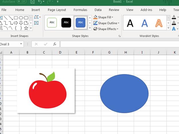
(A circle shape added to a spreadsheet)
The default style is applied to a shape, but a menu is shown after it has been added. In the image above, a circle was added to the same worksheet as the apple, and the active menu tab switches to "Format." You can change the shape to a different one or add styles to the shape. These styles are similar to the ones shown for the online picture added in the previous section. For instance, click the "Shape Effects" dropdown and take a look at the options. Notice that the "Shadow" option is also available for the circle. Click this option and select a preset shadow shown in the submenu. The selected effect is added to the shape.
(A drop-shadow added to an Excel shape)
Just like changes to images, you can also use the "Undo" button should you add a shape filter effect that you determine you don't want. The "Undo" button will reverse changes and revert back to the shape's original look and feel.
Formatting Shapes and Images
Resizing and adding effects to images are just a few formatting options, but when you work with spreadsheets that will be used in illustrations and presentations, you need a way to align and organize these objects.
With both the apple image and circle still added to your spreadsheet, move the circle to the same location as the apple. Notice that the circle is shown above the apple image.
(One object overlaps another image)
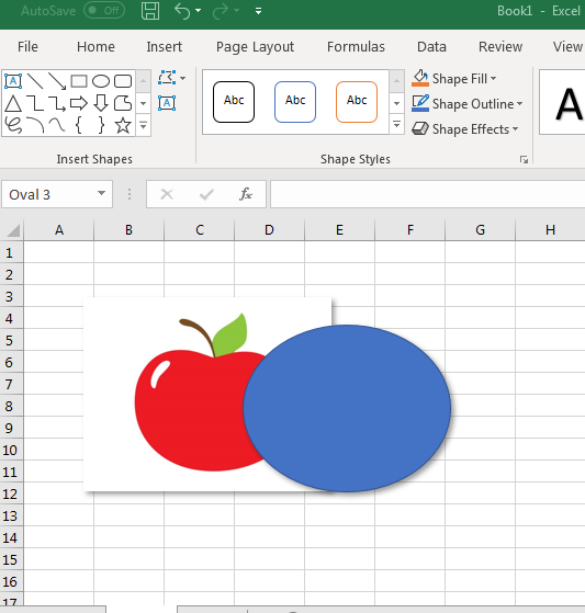
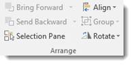
Image layers added to layers, and this is how you can understand the way image display in a spreadsheet. Since the circle object was added after the apple image, this second layer was added on top of the first apple image. If you add a third image to the document, it would display on top of the apple and the circle. You can change the way these layers are arranged in the "Format" tab.
If you've clicked away from any of the images, the "Format" tab option disappears from Excel's menu. Click the blue circle and notice that "Format" displays again in the menu. Click the "Format" tab in the menu and a category named "Arrange" is displayed with the other format functions.
The "Bring Forward" option takes a selected object and places it "on top" of other image layers. "Send Backwards" sends a selected object to the "bottom" of all other layers.
To test this feature, click the blue circle and then click "Send Backward." Notice that now the apple image displays in front of the circle.
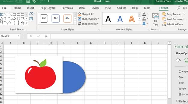
(The circle is arranged behind the apple image)
With Excel's styles and effects, you can add any premade image or shape and need no special software to edit objects. This saves you time as you create spreadsheets, and you don't need to edit images before adding them to your files. With Microsoft's online search for images, you don't even need to create your own. Instead, use Microsoft's Bing search engine to find an image and quickly add it to your spreadsheet. It's important to note that when a spreadsheet has images added to it, the file grows significantly larger and needs more hard drive space for storage.
Crop a Picture
When you crop a picture, you cut away the outer edge of the picture to create a new version.
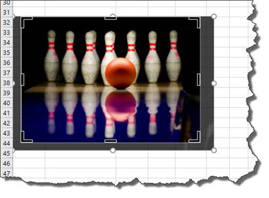
Let's crop the picture below.
Go to the Picture Format tab. If you don't see the Picture Format tab, double click on the image. Click Crop from the Size group.
Your cropping options are now displayed in the dropdown menu.
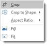
Select Crop.

As you see above, there are now black crop handles at each corner of the image and halfway across each edge. These crop marks look like "L" and dashes.
Click and drag your mouse on any of these marks. Click and drag inward on the image until you have cropped away the area you want to get rid of in the image.
The area you're cropping away is shaded in dark gray.
Click outside of the image to remove the cropped area.

Color
You can easily adjust the color of any image you place in your spreadsheets.
To do this, double click on the image.
You'll then see the Picture Tools Format Tab. Click the Color button:
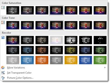
Choose the color effect you want to apply to your image.
Color Correction
You can also adjust and modify the colors in your image through color correction. Once again, go to the Picture Tools Format tab by double clicking your image.
Click the Corrections button.
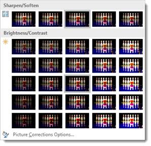
Choose a color correction.
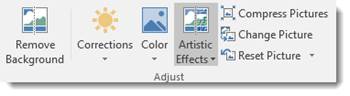
Artistic Effects
Just as you can use Photoshop and other photo editing software programs to add effects to your images, you can also use Excel for this.
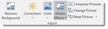
Double click your picture to bring up the Format tab, then click the Artistic Effects button.
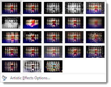
Choose the artistic effect that you want to apply to your image.
Rotating an Image
To rotate an image, we click the Rotate button in the Arrange group under the Picture Format tab.
Decide how you want to rotate it by making a selection in the dropdown menu:
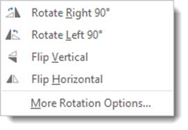
We're going to Rotate Right 90 degrees.
Excel rotates the image for us.

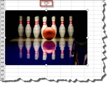
NOTE: You can also rotate images by selecting the image, then dragging on the arrow above the image. The arrow looks a lot like the Redo button.
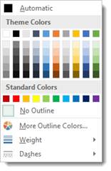
Changing the Borders of a Picture or an Image
The picture border tool is located in the Styles group on the Picture Format Ribbon in the Picture Styles group.
Border refers to the border around the outer edge of a selected element. To change the border of an image, you can click this button in the toolbar, and then select the desired color, weight (thickness), and style of the line.
Adding Styles to Images
In addition to adding borders to images, you can also add a style. A style can give the image a 3-D effect, add borders, shadows, and reflections.
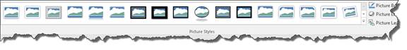
To add a style, select the image, then choose a style from the Pictures Styles gallery under the Picture Format tab.
Removing Backgrounds from Images
Although Microsoft Excel is a spreadsheet program, it also offers some photo editing tools, as we've already seen. Perhaps one of the most useful photo editing tools found in Excel 2019 is the background removal tool. This tool allows you to remove backgrounds from your images.
We are going to remove the background from our image:

To use this tool, double click on the image for which you want to remove the background. Click on the Remove Background button in the Adjust group under the Picture Tools Format tab.
When you click the Remove Background button, you will see the Background Removal tab appear on the Ribbon.
Your image's background � and possibly your image � will also change colors. Don't worry. This is temporary.
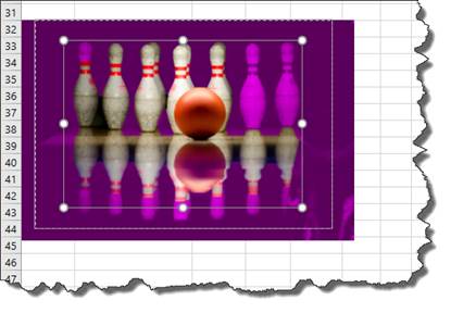
The areas that appear in purple are the areas that Excel 2019 has determined are background areas that it needs to remove. If there is purple on any areas of your image that you want to keep, you can drag the handles of the bounding box that appears over the image. Drag the handles outward to keep more of the image.
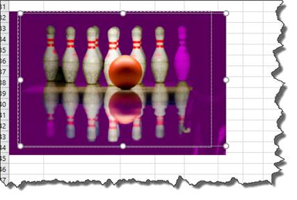
In the snapshot above, you can see we have dragged the handles outward. As we did so, more parts of the image returned to their regular color, which means those areas are not background areas. However, Excel is still recognizing a lot of the foreground image as background, and we need to change that.
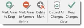
After you adjust the bounding box, if there are still areas of your image that are purple that are not supposed to be purple, go to the Background Removal tab in the Ribbon. Remember, any areas that are purple are considered background areas by Excel 2019.
Click the Mark Areas to Keep button.
Your cursor will turn into a pencil.
Simply click on any area that you want to keep.
You can also click on the Mark Areas to Remove to remove any areas that appear as foreground but should be background.
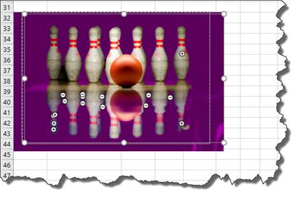
As shown in the snapshot above, a plus sign appears where you clicked areas to keep. Minus signs appear if you clicked areas that should be removed.
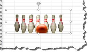
When you're finished, click the Keep Changes button in the Ribbon.
In our image below, we removed the background and then cropped the image.
Resize and Move Images
You can resize and move images after you insert them into Excel 2019.
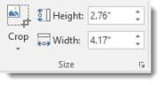
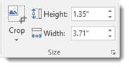
To resize images, go to the Picture Tools Format Ribbon. Go to the Size group and enter a size in inches for the height and width.
You can also resize a picture by dragging in or out on its handles on the bounding box in the spreadsheet.
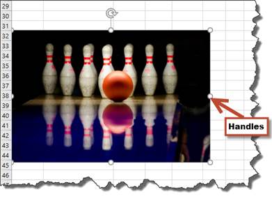
To move an image, click on the image so it's selected. Move your mouse cursor over the image. The cursor will turn into two arrows that look like a plus sign. Now, drag your image to its new location, then release
Compressing a Picture
You can reduce the file size of a picture by using the Compress Picture command. This reduces the resolution of the picture for quicker downloading and removes unnecessary information. For instance, when you crop a picture, the cropped portions of a picture are still stored in the file, they have only been "hidden."
The Compress Picture button is located under the Picture Format tab in the Adjust group.
Click the Compress Picture button.
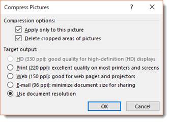
Choose the options you want, and click OK.The E-mail option reduces picture resolution to 96 dpi, or dots per inch. This helps increase the send/receive speed of your spreadsheet when you email it.
Reset Picture
Use the Reset Picture button on the Picture Format ribbon to reset the picture to its original size and format.
Adding WordArt
You might be familiar with WordArt from Excel's sister program Word. You insert WordArt into Excel much the same as you insert a picture.
Go to the Insert tab and select WordArt from the Text group.
You will then see the WordArt gallery.
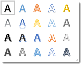
Select a style by clicking on it.
Click inside the box on your spreadsheet to type in your own text.

When you add WordArt, the Drawing Tools Format tab opens in the Ribbon.

From here, you can format your WordArt by applying a style, fill (the inside coloring of the letters, shape outline (the outline color of the letters), and even text and shape effects, such as drop shadow, reflection, etc.
Inserting Shapes
There are so many things that you can do to customize your Excel spreadsheet. One of those things is adding shapes.
To add a shape, go to the Insert tab and click the Shapes button in the Illustration group.
Select a shape from the dropdown menu.
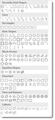
Select a shape. We've selected a cloud in the Callout section. Now simply click in the spreadsheet where you want the shape to appear:

You'll see a bounding box around the shape:

The little arrow at the top of the shape that looks like the Redo sign can be used to rotate the shape to the left or right.

You can drag on the handles (the little squares) to enlarge or reduce the size of the shape.

Double click the shape to bring up the Format tab on the Ribbon:

Shape and Text Effects
Text Effects and Shape Effects are visual effects that you can apply to word and shapes in your Excel 2019 spreadsheets. Shadow, glow, and reflection are examples of the visual effects that you can add. That said, when you add visual effects to your text or shapes, you want to select a visual effect that matches the look you want to create. You don't need to worry about what type of effect is.
To add visual effects to Word Art text, double click the WordArt to go to the Drawing Tools Format tab, then go to Text Effects in the WordArt Styles group.
To add visual effects to shapes, double click the shape to go to the Drawing Tools Format tab. Go to Shape Effects in the Shape Styles group.
You can then apply various visual effects to your text and shapes.
You can pick:
- Outline which will create an outline around the letters of your text or shape.
- Shadow which will add a drop shadow to your text or shape.
- Reflection which will create a reflection of your text or shape.
- Glow which will add a glowing effect to your text or shape.
- Bevel which will add a bevel to your text or shape.
- 3-D Rotation which will rotate your text or shape to give it a three dimensional effect.
- Transform (Text Only) transforms the shape of your text. By default, text goes from left to right in a horizontal line. When you transform your text, you can have it appear in a circular shape or as a wavy line.
By clicking on any of these effects in the dropdown menu, you can see the various options for the effect.
Create a Hyperlink
A hyperlink is a link to a website or location on the Internet � or even your computer if the person reading your spreadsheet has access to your computer files. To insert a hyperlink into a spreadsheet, go to the Insert tab, then the Links group. Click the Hyperlink button.

You'll see this window:
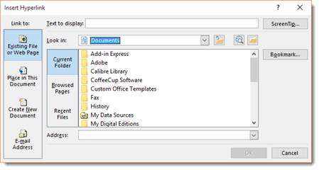
In the Text To Display field, enter in the text you want displayed in your spreadsheet. This will be the text people can click on to take them to the web page. It doesn't have to be a URL. You can type in the word "cow" if you want.
Choose what you want to link to. We've chosen a place in the spreadsheet.
Click OK when you're finished.
Embedding an Object
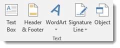
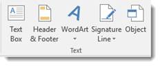
To embed an object into Excel 2019, select a location, then click the Insert tab, then the Object button in the Text group.

The Object dialog box will open.
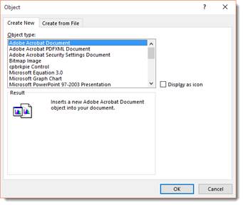
As you can see, you can now choose an object to embed. We're going to scroll down and embed a WordPad document.
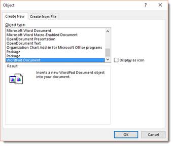
Click OK when you've chosen your object.
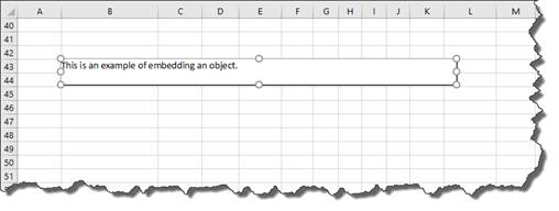
We now have a WordPad spreadsheet open on top of our spreadsheet.
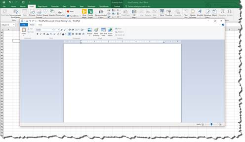
Start typing into the WordPad document.
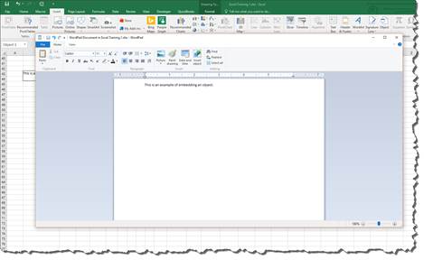
When you're finished, click the File tab in the WordPad document.
Select Exit and return to document.
The object is now embedded. You can resize, move, and even format the object.
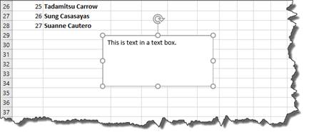
Textboxes
Sometimes, you don't want to type in a cell. Perhaps you have a picture that you need to add a caption for or you want to type instructions. For things like this, you create text boxes to enter in text. Text boxes can easily be moved, resized, and repositioned (along with the text inside them) to make creating a layout easy.
To create a textbox, go to the Insert tab and find the Text box button in the Text group.
Click the Text Box button.
The cursor changes to a downward arrow over your spreadsheet.
Simply click and drag to draw your text box. You do not have to draw it according to cells. In other words, you don't have to worry about starting at the top corner of one cell and dragging. You can put it wherever you want.

When you quit dragging and release your mouse, the cursor will appear in the text box.
Enter your text.
You can format the text in a text box the same way that you format a cell.