Objectives

 

 

You should already be familiar with rectangular (or Euclidean) coordinates: in three dimensions, we generally use x, y, and z as labels for our axes. This system uses fixed axes (in the context of vectors, the unit vectors have a constant direction). Although this coordinate system may be the most intuitive, it is not always the most convenient one for representing functions or points. In this article, we will introduce a simple alternative coordinate system: polar coordinates.

 

Introduction to Polar Coordinates

 

Consider some point P with rectangular coordinates (x, y). This point is shown on the graph below. (Note that (x, y) can also represent a vector r, which is also shown on the graph.)

 

 

 

Note that P resides on a circle that has a radius of length .

 

 

 

 

 

 

Here, following the results of our investigation into vectors,

 

 

 

 

 

 

Thus, we can narrow down the location of P by way of one number, the distance from the origin. But that still leaves a set of points on a circle, not the specific point P. Recall from trigonometry that we can use an angle measured relative to the x-axis to get a specific triangle--which, not coincidentally, corresponds with a specific point on a circle centered on the origin. Let's continue to call this angle θ.

 

 

 

 

 

 

Now, we have uniquely identified the location of the point P: it is located at a distance from the origin and an angle θ from the horizontal (x) axis. We can find any point on the plane using the coordinates (r, θ), where . These coordinates are called polar coordinates. (Note that unlike the constant unit vectors i and j that define locations in rectangular coordinates, the unit vector in polar coordinates changes direction with θ.) We have already related r to the rectangular coordinates x and y, but we can also do so for θ.

 

 

 

 

 

 

Note that we can use inverse trig functions to represent θ.

 

 

 

 

 

 

 

 

Now, the inverse tangent must be interpreted carefully, because the angle θ has the range [0, 2π) or (–2π, 0], depending on which way it is measured. But these ranges need not be limited as such--they are just what is necessary to define every point on the plane. No inconsistencies arise if we say θ has a range (-∞,∞); the only concern is that each point is defined by more than one set of coordinates. That is, in the case of our point P, it is located at (r, θ + 2nπ), where n is any integer. In other words, given the location (r, θ), if you go "around the circle" any number of complete revolutions, you end up at the same point. Thus, the location (r, θ) is equivalent (in some sense, at least) to (r, θ + 2π), and so on. We will not delve too deeply into this issue, however.

 

 

 

 

 

Another point of interest is converting from polar coordinates back to rectangular coordinates. This is easy if we simply apply trigonometry.

 

 

 

 

 

 

Thus,

 

 

 

 

 

 

 

We are thus able to convert back and forth between rectangular and polar coordinates.

 

 

 

 

 

Practice Problem: Convert the following sets of rectangular coordinates into polar coordinates.

 

 

 

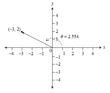
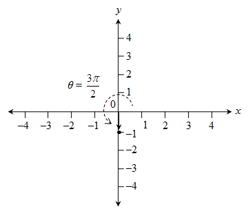
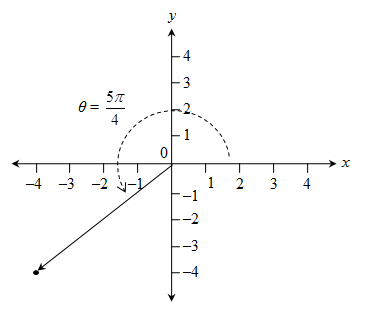
a. (1, 5) b. (-3, 2) c. (0, -1) d. (-4, -4)

 

 

 

Solution: To calculate r, simply use the Pythagorean theorem (). Then use the arctangent to calculate θ (that is, ). Be careful, however, to choose the correct value of θ in accordance with the location of the point! The coordinates below are in (r, θ) form; the values of r are exact, and the values of θ (in radians) are numerical estimates in some cases.

 

 

 

a.

 

b. (the point is located in the second quadrant of the graph--that is, the x coordinate is negative, but the y coordinate is positive)

 

 

 

 

 

 

c.

 

 

 

 

 

 

d.

 

 

 

 

The best approach to ensuring that you chose the correct angle is to convert the polar coordinates back to rectangular coordinates to see if they match; if not, you've either erred in calculating r or the angle θ.

 

 

 

 

 

Algebraic Relations in Polar Coordinates

 

 

 

As mentioned previously, certain algebraic relations have much simpler expressions in polar coordinates than in their rectangular counterparts. For instance, consider the equation of a circle of radius c. To express this relation in rectangular coordinates, we would need to write the following:

 

 

 

 

 

 

 

 

 

Here, c is a constant. (Note that this expression results from the Pythagorean theorem: , which we showed to be related to a circle of radius c in our discussion of trigonometry.) What about in polar coordinates? First, we can assume r is the dependent variable and θ is the independent variable; a function would then be written r(θ). In this case, the radius is always equal to c, regardless of the angle θ, so

 

 

 

 

 

 

This result is much simpler than the expression in rectangular coordinates! Of course, writing the expression for a horizontal line in polar coordinates can be extremely difficult, whereas it's a snap in rectangular coordinates: f(x) = a, where a is a constant.

 

 

 

Let's look at a really neat case involving an algebraic relation in polar coordinates: a spiral. Let's define a function r(θ) as follows:

 

 

 

 

 

 

A plot of this function is shown below. Note that the constant 2π simply governs how "tight" the spiral is. In this case, 2π is chosen simply to make some of the intercepts occur at simple numbers. Also note that θ here is measured in radians, not degrees. The graph shows the relation only for the θ domain [0, 4π]. We could, however, show any part of the domain (-∞, ∞).

 

 

 

 

 

 

We can make other interesting shapes by using trigonometric functions. For instance, consider the relation below.

 

 

 

 

 

 

The graph for this relation is shown below. Not coincidentally, the number of "lobes" in the graph is equal to the coefficient of θ in the argument of the sine function. This graph is for the θ domain [0, π].