The List Command is a feature that's new to MS Excel 2003.  Even though you could create lists in previous versions, the List Command makes it easier and quicker.

Lists in MS Excel are orderly rows of data, such as names, addresses, or even sales totals.  You can sort columns or rows into lists and they can be sorted, totaled, or tallied.

Creating a List

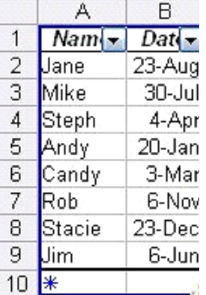
Neatness counts for everything in Excel, so the data in your worksheet should already be organized into neat rows and columns before creating a list.  Let's say you have already done that and you have a worksheet that looks like the one below with names and dates.

To make Excel see this data as a list, you'd click on any cell in the data area of the worksheet.  Then you'd go to Data>List>Create List.

When you do this, the data area will become active and you'll see the dialogue box pictured below.

This dialogue box confirms the area for the data and that your worksheet has column headers.  If it doesn't, that's okay.  Excel will create them for you.  Just uncheck the box.  (Column headers are the letters of the columns in the grayish box.)

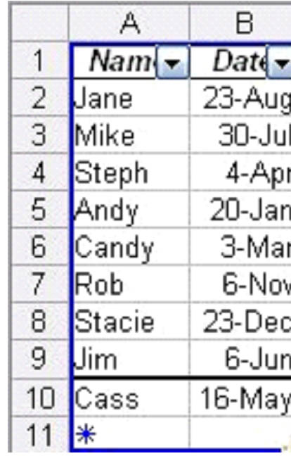
After clicking OK, the worksheet above now looks like this:

In addition, the List toolbar is now floating on the screen, if you don't already have it displayed in the toolbar area.

Note in the worksheet pictured above, that AutoFilter arrows are now in the header row and there is a dark blue line around the data to be used in creating the list.

The dark blue line signifies the data to be used in the list.  MS Excel 2003 allows you to have more than one list, so the dark blue border shows you where each list is located.  If you click outside the list, the dark blue will change to light blue.

Note:  The AutoFilter arrows were added for you.  Earlier versions of Excel made you add them yourself.

Inserting Rows and Columns into a List

The asterisk at the bottom of the list is where you would insert rows.  To insert a row, just type the data where the asterisk is located.  After you do, the asterisk will be located beneath your new row so that you can continue to add data. 

If you click outside the list area, the asterisk will disappear. 

You can add a column by typing in the column to the right of the list area.  MS Excel will automatically expand the list area for you.  We'll learn how to insert rows and columns into the middle of the list area later in this article.

Adding Up Values

To add up value in a list, you must use the Toggle Row button on the List toolbar.  It looks like this:

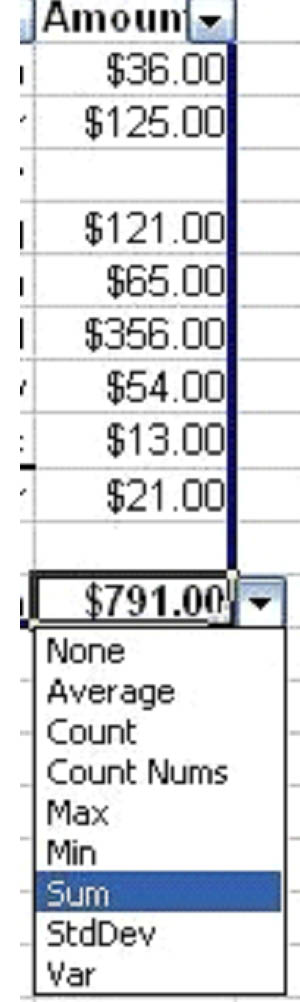
The Toggle Row button automatically totals the last column in the list.  To get the total for Column see in the list above, you would just hit the Toggle Row button and Excel would produce a total.  See the snapshot below.

If Column C had data that couldn't be totaled, like a list of names, it would tally the number of names instead. 

However, that doesn't mean we have to produce a sum for the last column.  Since it was numbers, MS Excel automatically gave us the sum, but we have other choices Excel lets us make.  Click on the cell that gives the total ($791.00) and an arrow will appear.

We're going to choose, for this example, to average the numbers rather than producing a sum.  We'd select Average.  The average of all the numbers in Column C would then appear in the total box instead of the sum.

Later in this article, we'll learn how to totals on columns other than the last one.

Sorting Lists

Any column in your list can be easily sorted by clicking on the AutoFilter arrow beside the heading and choosing one of the selections.  Let's say, for this example, we wanted to sort the names alphabetically.

First, we'd click the AutoFilter arrow beside the word Name.

Then, we'd click on Sort Ascending.  

When we click on Sort Ascending, all names are alphabetized.

 

To sort more than one column at once, you'd go to Data>Sort.  This dialogue box will appear:

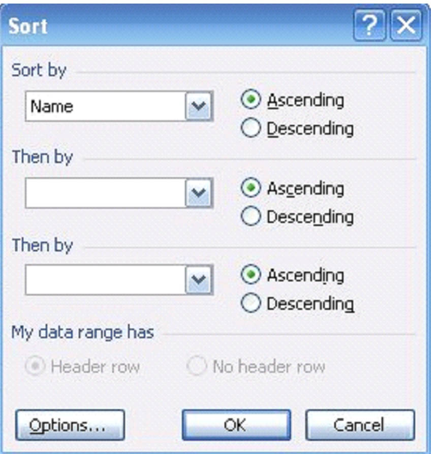
You'd then choose the sort order for your list and click OK.

Using Filters to Sort Lists

Filtering data in your list is as easily as sorting it.  Simply click on the AutoFilter arrow and select the data by which to filter the list.

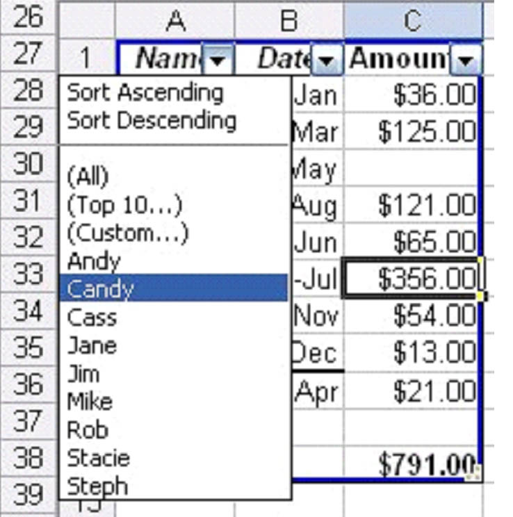
We've chose the Name column and to filter the data using Candy.

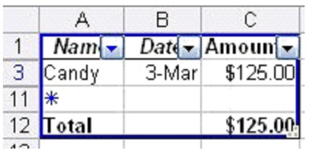
Only Candy's information is showing.  The rest has been filtered out.

Using List Border to Expand a List

Click and drag the lower right hand corner.