In this article, we look at one-sample Student's t-tests as a method for determining whether a sample mean deviates in a statistically significant manner from a known or predetermined population mean. This article relies heavily on statistical hypothesis testing.
Key Terms
o One-sample t-test
o Normally distributed
o Normal distribution
o Bell curve
o Gaussian distribution
Objectives
o Learn and apply hypothesis testing procedure to the one-sample Student's t-test
Resources
o A table of values for the Student's't distribution is available at http://www.itl.nist.gov/div898/handbook/eda/section3/eda3672.htm
Let's Begin!
In our discussion of cross tabulations, we considered hypothesis testing as a method for determining if the variables in the cross tabulation were in some manner related. Hypothesis testing has numerous other applications as well--we need only choose null and alternative hypotheses, an appropriate test statistic, and a statistical significance. Using tables of values for that test statistic, we can then determine whether to accept or reject the null hypothesis.
In this and the next article, we look at Student's t-tests, which are applications of the hypothesis testing procedure that allow us to determine whether a sample mean deviates significantly from either a known mean value or another corresponding sample mean. In this first article, we consider one-sample t-tests; in the next article, we consider two-sample t-tests.
One-Sample Student's t-Test
One goal of statistics is to determine whether some sample statistic deviates in a statistically significant manner from a predetermined or otherwise known value. For instance, a machine shop might require parts with a certain mean size. A machine that produces the parts is unlikely to produce a set of parts with exactly the predetermined mean, but that deviation may not be statistically significant. (In other words, the machine may be producing parts with size variations that are within the range of what we would expect, given that neither machines nor materials are perfect.) In this case, the one-sample Student's t-test can help a machinist determine if the machine is working within acceptable parameters, or if the mean part size produced by the machine is deviating significantly from the required mean. The machinist need only an understanding of hypothesis testing, a table of Student's't values, and a data set of measurements for a sample of parts from the machine.
The one-sample Student's t-test (which we will often refer to as simply the one-sample t-test) can be employed only under certain fundamental assumptions about the data. First, the variable being tested (the mean size of parts from a machine, if we follow our example from above) must be normally distributed . This is to say that if we collected a large (ideally, infinite) number of sample values and plotted the frequencies graphically, we would find that the graph is a normal distribution (also known as a bell curve or Gaussian distribution ). A general normal distribution is shown below, with the associated mean value and standard deviation labeled as μ and σ, respectively.
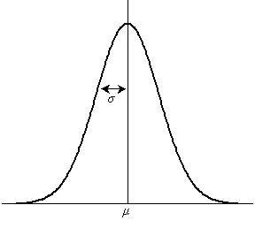

Many variables with practical significance are distributed normally. We will not consider this matter further, but we will assume we have some method of determining whether a variable is normally distributed.
Another assumption of the one-sample t-test is, of course, that the population mean is known (or, as in the case of the machine shop example, is predetermined). We must have a standard against which we are comparing our sample values; that standard is the population mean, whether it is determined arbitrarily, as with the required mean size of a metal part, or it is determined theoretically on the basis of other information. Again, in either case, we have a known value against which we can compare a value calculated on the basis of a sample.
Finally, the one-sample t-test assumes that our sample data are taken randomly from the population. The test does not work if data values are "cherry picked," since this kind of selection can skew the sample mean in one direction or another. Thus, for instance, the machinist might determine that he intends to use the first 30 parts from the machine as a sample for the test-as long as he sticks to this plan, he has taken 30 samples at random.
Procedure for the One-Sample Student's t-Test
The first step of the procedure for the one-sample t-test is to choose a null hypothesis (and, correspondingly, an alternative hypothesis). In general, the null hypothesis has the following form:
H0 = The sample mean ![]() is the same as the population mean μ.
is the same as the population mean μ.
Logically, the alternative hypothesis is then
Ha = The sample mean ![]() differs from the population mean μ.
differs from the population mean μ.
The next step is to choose a statistical significance-the value we labeled α in our previous discussion of hypothesis testing. A value of α = 0.05 is common; we will typically use this value. Some situations, however, call for a value such as 0.01.
Assuming we know the sample mean and population mean that we wish to test, all that remains is determining a test statistic and the corresponding critical value. Our test statistic is the Student's't value, the formula for which is given below, where s is the sample standard deviation and n is the sample size (the number of values in the sample data set).
![]()
For the purposes of the one-sample t-test, the number of degrees of freedom in the problem is n – 1 (this is also the same as the "sample size" used in the estimator for the standard deviation).
Finally, we can find the critical value c on the basis of our choice of α and of the number of degrees of freedom in the problem by consulting a table of Student's't values. As with the chi-squared tables, the Student's't tables often list values according to 1 – α rather than α.
At this point, we can now put our knowledge to work using the one-sample Student's t-test.
One-Sample Student's t-Test Example
Let's continue with our example of the machinist in the machine shop. Assume that he needs parts with a mean size of 4.32 centimeters. He then uses the machine and produces 10 parts, whose sizes are listed below. (Assume also that the size of the parts is a normally distributed variable-this assumption is likely valid in a practical situation.)
{4.26, 4.13, 4.53, 4.39, 4.27, 4.35, 4.21, 4.58, 4.09, 4.10}
The sample mean, ![]() , is
, is
![]()
Because the machinist needs a mean of 4.32 centimeters, we define our population mean as this value (μ = 4.32).
Let's choose a significance value of α = 0.05. The number of degrees of freedom in the problem is 10 – 1 = 9. We can then determine the critical value, c, from the table of Student's't values.
c = 1.83
We need only calculate the test statistic at this point. First, we need to calculate the sample standard deviation, s.
![]()
![]()
The test statistic is
![]()
But since we are really only interested in the absolute value of the statistic, we use t ≈ 0.555. Since t < c, we do not reject our null hypothesis--the sample mean does not deviate significantly from the desired mean.
Practice Problem: The population mean for height of people in a particular city is 67 inches. The following set of sample data are collected randomly. Determine if the sample mean deviates significantly (to a 0.05 significance level) from the population mean.
{64, 67, 73, 75, 69, 70, 62, 75, 72, 68, 71, 69}
Solution: Our null hypothesis is that there is no difference between the sample mean and population mean. Let's now calculate the mean and standard deviation of the sample.
![]()
![]()
![]()
Our problem has 12 – 1 = 11 degrees of freedom, and the statistical significance is α = 0.05. The critical value, on the basis of the table, is
![]()
The Student's't value (our test statistic) is
![]()
Since the value of t exceeds the critical value, we must reject the null hypothesis and proceed on the assumption that the sample mean deviates significantly from the population mean. This could mean, for instance, that the sample was chosen in a poor manner.


