Key Terms
o Scatterplot
o Marginal distribution
o Independent (random variables)
o Dependent (random variables)
Objectives
o Recognize and understand how to interpret bivariate distributions
o Understand what a marginal distribution is
o Differentiate between dependent and independent random variables
In this article, we will expand out discussion to more than one variable (we will limit the discussion to just bivariate data--two random variables, which we can label as X and Y) which allows us to consider more advanced topics in statistics such as correlation and regression analysis. We will introduce some of the terms and concepts that will allow us to focus on these advanced topics.
Bivariate Distributions
To reiterate, we will focus only on bivariate data rather than data with three or more variables; although the discussion is limited in this way, the concepts can easily be extended to many more variables (although the mathematics may get progressively more involved). When we dealt with a single random variable, X, we were able to express the associated data in a single dimension: we simply used a list or column of data values. If we add a second random variable, Y, then we must express the associated data in a two-dimensional manner. Such an expression requires a list combining two data values, as with the example below:
{{1.0, 15.3}, {5.0, 18.2}, {7.0, 25.8}, {4.0, 22.0}, {3.0, 18.9}, {2.0, 13.0}.}
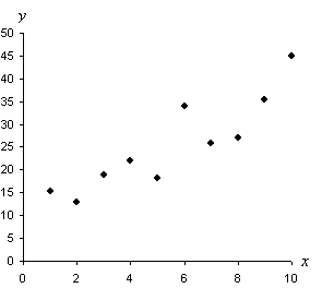
Note that data in this case is presented in pairs (of the format {X, Y}), rather than as single values. When using a table, we would list the data values using two separate columns. If the data are not repetitive (that is, the frequency of each data point is unity--or very close to unity), then a scatterplot is one way to display the data. A scatterplot simply constructs a graph with two axes and places a dot at each point whose coordinates correspond to one of the pairs of data values. The example data below (and a few extra points) are shown in the scatterplot below. Note that a scatterplot allows us to look for possible trends (or relationships) in the data.

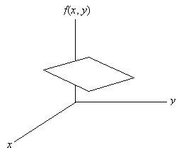
Even though we are examining pairs of data values, each pair can still have an associated frequency (and, consequently, a relative frequency or probability). We can plot the probability function using a three-dimensional graph (in the case of univariate data, the plot of the probability function was a two-dimensional graph). A portion of a three-dimensional surface is shown in the graph below, where x and y correspond to random variables X and Y, respectively, and f(x, y) is the probability density function.

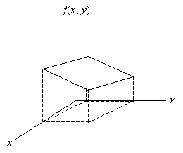
A bivariate distribution, like a univariate distribution, can be either continuous or discrete. When calculating probability for a continuous distribution (such as P(X ≤ a, Y ≤ b), for example), we must calculate a volume, instead of the area that we calculated for a univariate distribution. Again, an exact calculation generally requires integral calculus, but some cases can be simplified. The volume that we would calculate for the distribution above is shown in the graph below.

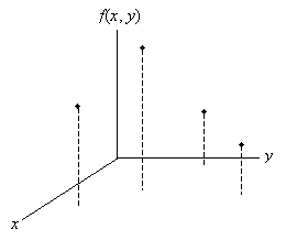
For a discrete distribution, such as that shown below, calculating a probability simply involves adding the relative frequencies of each outcome in the event of interest. In the following graph, f(x, y) is the probability (relative frequency) function.

Marginal Distributions
Because dealing extensively with continuous distributions requires knowledge of integral calculus, we will limit our discussion to discrete distributions for the remainder of this article. Given the discrete random variables X and Y and probability distribution f(x, y), we may be interested in determining the probability of a particular value for one of the variables regardless of the value of the other variable. For instance, in a situation where a statistician has collected age and income data for a population, he may want to find the probability that a random person has a particular income range, regardless of age. To do this, the statistician can use the marginal distribution for age. A marginal distribution is the probability distribution for a particular random variable where the other random variable takes on an arbitrary value. Using our X and Y notation, we can define f1(x) as the marginal distribution of X with respect to f(x, y) and f2(y) as the marginal distribution of Y with respect to f(x, y). We can express these functions algebraically as follows:
f1(x) = P(X = x, Y arbitrary)
f2(y) = P(X arbitrary, Y = y)
For a particular value X = x, the function f1(x) is the sum of f(x, y) over all values of y for X = x. This summation eliminates the influence of the variable Y by calculating the probability that X = x regardless of the value of Y. We can thus further define f1(x) and f2(y) as follows.
f1(x) = ![]()
f2(y) = ![]()
(For continuous distributions, the summations would be replaced with integrals.) Based on these definitions, we can determine whether the two variables X and Y are dependent or independent. Random variables X and Y are independent if they satisfy the expression
f(x, y) = f1(x) f2(y)
Otherwise, the random variables are said to be dependent. Conceptually, independent random variables are variables whose individual probability functions can each be expressed without reference to the other variable. Thus, for example, if X corresponds to the outcome of rolling a red six-sided die and Y corresponds to the outcome of rolling a green six-sided die, X and Y are independent because the value of X has no bearing on the value of Y (and vice versa).
Practice Problem: Two fair six-sided dice are rolled-one die is green and the other is blue. If X is the value rolled for the green die and Y is the value rolled for the blue die, what is the probability distribution f(x, y), where X = x and Y = y?
Solution: This problem requires that we apply several different concepts. First, we know that the random variables X and Y are independent because the number rolled for one die has no effect on the outcome for the other die. As a result, we need simply calculate the marginal distribution for each die and then find the product. Given that each die is fair, the probability of rolling any number one through six is 1/6 for each die. Thus, the marginal distributions are
f1(x) = f2(y) = 1/6
The bivariate probability distribution is then
f(x, y) = ![]()
This distribution is uniform-every outcome (for instance, {1, 6}, {6, 1}, {2, 3}, etc.) has an equal probability.
Practice Problem: Random variable W is the number drawn from a hat containing papers marked 0 through 99, inclusive. Following the drawing, the number is set aside. Random variable Z is the number drawn from the hat subsequent to the first drawing. Determine if these random variables are independent.
Solution: Because the first drawing reduces the sample space of the second drawing (the number is not replaced after the first drawing), the probability distribution of Z is directly affected by the value of W. (For instance, if W = 0, then the probability that Z = 0 is zero. If W = 1, then the probability that Z = 0 is 1/99.) Thus, the random variables are dependent.


