How to Calculate Probabilities for Normally Distributed Data

Key Terms

o Normal distribution

o Gauss distribution

o Bell curve

o Standardization

o Z-score

o Standard score

Objectives

o Recognize the normal distribution and its fundamental characteristics

o Know how to standardize a random variable using the Z-score

o Calculate probabilities for normally distributed data

Resources

o A table of values for the standard normal distribution is available at http://www.mathsisfun.com/data/standard-normal-distribution-table.html. (Be aware that this table is slightly different than the type of table used to solve the problems in the article--the difference is discussed, however.)

A number of different types of specific distributions have various applications, but one distribution in particular is heavily used (and well known) across a wide range of areas. This distribution is known as the normal distribution (or, alternatively, the Gauss distribution or bell curve), and it is a continuous distribution having the following algebraic expression for the probability density.

In this formula, μ is the mean of the distribution and σ is the standard deviation. The general form of the normal distribution is shown below; note the "bell-curve" shape of the graph, and note that the distribution is symmetric about the mean (peak).

Because this distribution is continuous, integral calculus is required to directly calculate associated probabilities. Nevertheless, because the normal distribution applies to so many different situations, tables containing probabilities for ranges of values are readily available. Furthermore, the distribution can easily be scaled to conform to the particular mean and standard deviation of interest. Although you need not fully understand the following notation, the probability P(X ≤ x) can be written as

This expression, which calculates the area under the curve from the extreme left (negative infinity) to x = c, refers to the shaded region shown below.

We can also calculate probabilities of the form P(a < X ≤ b)--in such cases, the shaded region would be more limited. Recall that a probability for a distribution is associated with the area under the curve for a particular range of values. As such, the area under the entire normal curve (which extends to positive and negative infinity) is unity.

It is important to note that this discussion applies mainly to populations rather than samples. The continuous normal distribution cannot be obtained from a sample (because it would require an infinite number of data values).

Z-Scores and the Normal Distribution

Interested in learning more? Why not take an online Statistics course?

Given a situation that can be modeled using the normal distribution with a mean μ and standard deviation σ, we can calculate probabilities based on this data by standardizing the normal distribution. Note in the expression for the probability density that the exponential function involves . Let's define this expression as z; this is also sometimes called the Z-score or standard score. Using techniques of integral calculus, we can show that

In the above expression, . Out of this transformation falls the standard normal distribution below:

The graph of this function is shown below.

Note that the standard deviation of the standard normal curve is unity and the mean is at z = 0. The peak of the curve (at the mean) is approximately 0.399.

You might be wondering at this point why we have brought in all the complicated mathematics and seemingly pointless changes of variables. Nevertheless, this process has a particular purpose: because we can standardize a data set from a normal curve with a particular mean and standard deviation to a standardized normal curve with a single mean (zero) and standard deviation (unity), we need only a single table to calculate probabilities for any normal distribution. Thus, regardless of the details of the problem, we can calculate probabilities for any normal distribution using the standardized distribution. This is a powerful result that allows even those who do not understand integral calculus to calculate probabilities for normally distributed data.

Using Standard Normal Distribution Tables

A table for the standard normal distribution typically contains probabilities for the range of values –∞ to x (or z)--that is, P(X ≤ x). This probability is the same as

Graphically, this probability is also equal to the shaded area shown below.

Typical tables provide probabilities for x values ranging from zero up to three or four (at which point the probability becomes extremely close to unity). What if we want to calculate probability P(X > x), which corresponds to the non-shaded area in the graph above? Because the probabilities P(X ≤ x) and P(X > x) span the entire sample space (–∞ < x < ∞), P(X ≤ x) + P(X > x) = 1. Then,

P(X > x) = 1 – P(X ≤ x)

So, we can still use the tables-look up P(X ≤ x) and then subtract this value from unity. What if we want P(X ≤ –x)? Recall that the distribution is symmetric; thus,

P(X ≤ –x) = P(X > x)

Finally, we might want to calculate the probability for a smaller range of values, P(a < X ≤ b). First, we calculate P(X ≤ b) and then subtract P(X ≤ a). The graph below helps illustrate this situation.

Thus, we are able to calculate the probability for any range of values for a normal distribution using a standard distribution table.

Data tables for the normal distribution can be found in many mathematics texts that deal (even lightly) with statistics and in many math reference books, as well as on the Internet (simply do a search for "normal distribution table" or "standard distribution table" using your favorite search engine). Not every table will present the data in the same way, however; typically, the table will include a plot of the standard normal distribution that shows the area (probability) associated with a particular value. In some cases, the area might be the following:

Since the normal distribution is symmetric about the mean, the area under each half of the distribution constitutes a probability of 0.5. The probability shown above is simply P(0 < X ≤ x)--you can likewise manipulate the results as necessary to calculate an arbitrary range of values

Practice Problem: The lifespans of people in a certain city constitute a normal distribution with a mean of 72 years and a standard deviation of 6 years. What is the probability that a randomly selected person from the city will live more than 75 years?

Solution: Let's assume that the random variable X corresponds to the lifespan of a person selected at random from the city mentioned in the problem. We therefore want to calculate P(X > 75). To do so, let's first calculate the Z-score of 75 years. Note that the mean μ of the distribution is 72 years and the standard deviation σ is 6 years.

We know that the probability P(X > 75) is equal to 1 – P(X ≤ 75), so we can use a table to find P(X ≤ 75). This result is equal to P(Z ≤ 0.5) (where Z is the standardized random variable). The table states that

P(Z ≤ 0.5) = 0.6915

Now we can calculate P(X > 75).

P(X > 75) = 1 – P(X ≤ 75) = 1 – P(Z ≤ 0.5) = 1 – 0.6915 = 0.3085

Thus, a randomly selected person from the city has a 0.3085 probability of living more than 75 years.

Problem: A scientist is measuring the speed of a projectile launched from a newly designed device. The mean speed of the projectiles is known to be 315 meters per second with a standard deviation of 11 meters per second. What is the maximum speed for 95% of the projectiles?

Solution: This problem reverses the logic of our approach slightly. We want to find the speed value x for which the probability that the projectile is less than x is 95%--that is, we want to find x such that P(X ≤ x) = 0.95. To do this, we can do a reverse lookup in the table--search through the probabilities and find the standardized x value that corresponds to 0.95. The standardized value is 1.645 (note that it is sometimes necessary to approximate through interpolation, since the table cannot cover all possible decimal values). We now need to convert to a speed.

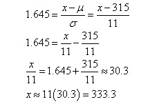
Thus, 95% of the projectiles have a speed of less than or equal to about 333.3 meters per second.

Practice Problem: For normally distributed data, what is the probability that a random experiment will yield a value within one standard deviation of the mean?

Solution: Although we are not given particular values for the mean and standard deviation of the data, we can still rely on the standardized normal distribution to make a general statement about all normal distributions. Recall that the standard deviation of the standard normal distribution is unity. Thus, we want to calculate the probability P(–1 < Z ≤ 1). We can also express this probability as

P(–1 < Z ≤ 1) = P(Z ≤ 1) – P(Z ≤ –1) = P(Z ≤ 1) – [1 – P(Z ≤ 1)]