Objectives

When we look at the graph of a function, one question we might ask regards the slope of the function at a given point. We can answer this question through differentiation of the function. Another question we might ask regards the area of the region under the curve. If we're dealing with a line, we can simply apply basic geometry, as in the example below.

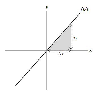
Say we wanted to calculate the area under the function f(x) (meaning the area between the function and the x-axis) for the region defined between x = 0 and x = ∆x. This region is shown as the shaded area in the graph above. Here, we can simply use the formula for a triangle, and we'll call F(x) the area under f(x) between 0 and x. (So, F(∆x) is the area under f(x) between x = 0 and x = ∆x.)

Simple enough. But what if the function f isn't linear?

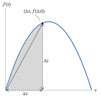
In this case, our use of triangle geometry at best gives us an approximation of the area, but certainly not an exact result. So, what are we to do if we want to calculate this area exactly?

You might already be thinking that we should try using more than one shape to improve the accuracy of the result. Let's try that, but instead of triangles, let's use a simpler basic shape: a rectangle. Obviously, a single rectangle isn't sufficient, so let's start with several. Note that we make some small notation changes below.

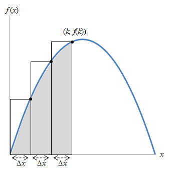
This is still a very rough approximation of the area of the region under the curve, but it is a start. This region is between x = 0 and x = k. Note several characteristics of these rectangles: First, for simplicity, they have the same width: ∆x, which obeys the relation

where n is the number of rectangles (three in the above case). Second, the height of each rectangle is the value of the function on its "right side." That is, the height of the mth rectangle is f(m∆x), as the graph illustrates below.

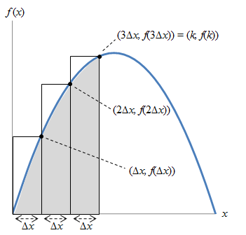
Now, following the same pattern, let's increase the number of rectangles.

In this case, we have six rectangles, where

We can continue increasing the number of rectangles indefinitely. As we do so, the white area of the rectangles (the portion not in the shaded region) will decrease, which means the accuracy of our estimate will improve.

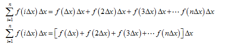
Let's now write an algebraic expression for the area estimate using summation notation (recall our discussion of series-this is a finite series). The area of the ith rectangle is just the product of its width, ∆x, and its height, f(i∆x).

For calculating the area under the curve from 0 to some arbitrary x value,

where, again, n is simply the number of rectangles we use. The sum is one type of Riemann sum. In general, Riemann sums can "position" the rectangles so that the curve intersects them at different points on the top side. We consider just one fairly simple case.

Now, if the number of rectangles (n) goes to infinity, we should end up with the exact area under the curve between 0 and x. That is, applying what we learned about limits to the Riemann sum,

Let's look at a specific simple case: .

Now, let's say we want to find an exact expression for F(x). Below is an illustration for f(x).

Let's start with the limit of the Riemann sum. Remember, as we saw above, this expression takes n rectangles and places them side by side to cover the grey area as closely as possible. In the limit, the number of rectangles, n, approaches infinity (meaning their width approaches zero).

Now, apply the function definition.

Remember that

So,

Because x is an arbitrary unknown with no relation to n or i, we can move it "outside" both the sum and the limit (don't worry if you're not entirely sure why this is the case--just try to follow the argument).

Furthermore, because n is a constant that is independent of i, we can move it outside the sum (but not outside the limit). (Again, you may be a little suspicious of this step. You have all the tools necessary to prove it to yourself, if you want--but for our purposes, we'll just assume it is justified.)

Now, we'll make one last leap that we'll just assume is justified:

 You can test this for various values for n to help convince yourself it works. But proving it for all values of n requires mathematical induction. But let's assume this is true and plug the result into our above expression.

Now, simplify and apply the limit.

As n approaches infinity, all but the first term in parentheses approach zero.

We now have an expression in x that represents the area under the curve of f(x) between 0 and x. What we have done here is perform integration. The result of the process is called the integral of f(x). Because the Riemann sum in this case involves an infinite series of infinitesimally small rectangles, we change the notation slightly:

As with derivatives, ∆x becomes dx, since this "width" is infinitesimally small (i.e., it approaches zero). The strange "S" shape stands for "sum." We can also write the integral as

Here, 0 and x are the limits of integration. We can also calculate integrals for arbitrary portions of the curve-it need not be just 0 to x.

Not coincidentally, it turns out that if we apply our differentiation process to our derived F(x) above, we get the following:

In other words, the derivative of the integral of f(x) is f(x)! For this reason, the form of the integral above is also called the antiderivative.

Although this derivation of the integral may be a little murkier to you than our discussion of differentiation (it is certainly a more complex topic), you should nevertheless have a decent understanding of where the integral comes from and what it means, even if you're a little unsure about the mechanics of the math.