Key Terms
Objectives
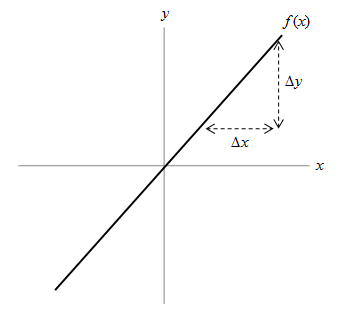
We know from basic algebra that a line has the form f(x) = mx + b, where m is the slope. We measure the slope as the distance traveled up (along the vertical axis) divided by the corresponding distance traveled across (along the horizontal axis): this is what we call "rise over run." We can also call the rise ∆y, since it is the change in y; the run we can call ∆x, since it is the change in x. Then,
![]()
A line has the same slope everywhere. It doesn't matter what size of ∆x we choose or where we choose it; the corresponding ∆y will yield the same value of m.
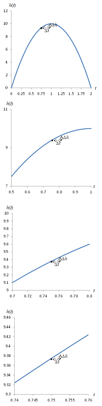
The slope m is also the rate of change of the function f with x. Let's say f was the vertical position of a rocket and x was time. The vertical speed (rate of change of height with time) of the rocket is m. But what if we were looking at the height of a ball thrown straight up into the air? The height h of the ball (in meters) at time t (in seconds) is a parabola, such as that shown below. Note that gravity causes the upward speed of the ball to slow and then reverse--that is, it eventually falls back to the ground.
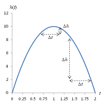
In the graph, we can see that our slope measurement is different depending on where we choose ∆t and on how large ∆t is. How are we to resolve this difficulty? How can we measure the slope of a nonlinear curve?
To answer that question, let's select a location at which we want to find the slope. Let's then "zoom in" on that point.
What you may be noticing is that as we magnify the portion of the curve around the point, the curve starts to look more and more like a line! As it turns out, if we use "infinite" magnification, the curve is actually a line. Try to imagine two adjacent points on a curve: the distance between them is essentially zero, but they do not occupy the same place. (If the distance between two adjacent points is nonzero, then we could fit more points between them, and they wouldn't be adjacent!) If we can find the slope of the curve by looking at these two adjacent points, we can find the slope of the curve at a given location. Let's look at this in terms of ∆t and ∆h on the graphs above.
In the above progression, ∆t gets smaller and smaller--as does ∆h. Let's apply what we know about functions to see if we can get something useful out of this result. Let's consider the general case of a function h(t)--not necessarily the function above, but we'll stick with the same notation for now. Let's call the slope of this function h'(t).
![]()
Now, note that the point of interest has coordinates (t, h(t)); this is the point at which we want to find the slope. The differences ∆t and ∆h give us the point (t + ∆t, h(t) + ∆h), which is shown below.
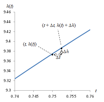
Note also that
Thus,
![]()
We can then rewrite the slope of the curve at point (t, h(t)) as follows.
![]()
As we observed before, a curve looks more like a line the more we magnify it around the point of interest. And as we did so above, we made ∆t get smaller and smaller. Let's now apply what we learned about limits. We want ∆t to get so small that we are looking at the slope calculated using two adjacent points on the curve. The distance between these points is zero. So, let's take the limit of the slope as ∆t approaches zero--in the limit, this will give us the slope of the curve at the point (t, h(t)).
![]()
Clearly, however, we can't evaluate this by just substituting 0 directly for ∆t; we'd end up dividing 0 by 0. So, let's consider a simple example: a basic parabola (similar to the function we looked at above). Let's use ![]() .
.

We want to find the slope of h at an arbitrary point t. Let's apply our slope limit to this function.
![]()
Simplify the result:
![]()
![]()
Now we have eliminated the problem of dividing by zero--the result is simply a polynomial. We know from our discussion of limits that we can just substitute 0 for ∆t. The result is a new function:
![]()
So, the slope of h(t) at any point t is simply 2t. Note that the slope varies with the value of t. What we have done here is determine the derivative of the function h(t): the derivative is simply the slope or rate of change of the function with respect to its independent variable. The process of calculating a derivative is known as differentiation. And to show that we are dealing with infinitesimally small distances between adjacent points in the slope calculation, we replace ∆ with d.
![]()
This form can also be expressed as follows:
![]()
In words, this is called the derivative of h(t) with respect to t.
Time does not permit us to go into heavy detail regarding derivatives for different functions, but you should now have a basic understanding of the derivative--one of the fundamental tools of calculus.
Practice Problem: Calculate the rate of change of the function ![]() at the following points:
at the following points:
a. x = 0 b. x = 1 c. x = 2 d. x = -2
Solution: Let's look at the graph of the function to help make sense of the results.
Remember, the derivative of f(x) with respect to x is the rate of change of that function at x. Following the results of the lesson, we know that
![]()
Now, we need only evaluate f '(x) at the given values to find the rate of change of f at those points.
a. x = 0 : f '(x) = f '(2) = 2(0) = 0
This result makes sense because the function is "flat" at x = 0.
b. x = 1 : f '(x) = f '(1) = 2(1) = 2
Here, the function is increasing.
c. x = 2 : f '(x) = f '(2) = 2(2) = 4
In this case, the slope of the function is increasing: it is growing at a faster rate as x increases.
d. x = -2 : f '(-2) = f '(-2) = 2(-2) = -4
The function is symmetric about the x-axis. Note that on the left side of x = 0, the function is decreasing, which is why its derivative is negative for values on this side.