Key Terms
o Random variable
o Probability distribution
o Discrete
o Continuous
Objectives
o Understand how algebra can be used in probability and statistics
Algebra in Probability
Probability concerns such considerations as the chance that a tossed coin will land heads up or tails up and the chance that a particular number will come up when a die is rolled. Although often such problems can be solved without reference to algebraic functions or variables, algebra can still be a crucial tool in analyzing more complicated problems. For instance, let's say we want to know how to calculate the probability that three tosses of a loaded coin will result in three heads. A "loaded" coin is a coin that is not fair (that is, a coin that has an equal chance of landing heads up or tails up). Let's say the probability that a particular coin toss will land heads up is h, where h ≤ 1. We can define a function p(h) that gives us the probability of three heads in three tosses as follows.
p(h) = h3
(For instance, if h = ![]() , then only one out of three tosses on average will be heads up. Only one in three tosses after that instance of heads up will likewise be heads up; therefore, we multiply the probabilities.) Given our definition of h, we can also define a function q(h) that gives us the probability that three tails are obtained in three tosses.
, then only one out of three tosses on average will be heads up. Only one in three tosses after that instance of heads up will likewise be heads up; therefore, we multiply the probabilities.) Given our definition of h, we can also define a function q(h) that gives us the probability that three tails are obtained in three tosses.
q(h) = (1 – h)3
These functions allow us to make a general analysis of probabilities associated with tossing a coin without knowing the specific probability of getting a head or tail in a given toss.
Because algebra allows us to use the concept of a variable, we can apply this in probability theory by using a random variable, which is a parameter or event (such as a coin toss) that has a random or unknown outcome. We might therefore assign the symbol X to the roll of a die. We can also create a probability distribution that shows us graphically the probabilities of the potential outcomes of a roll. Such a probability distribution is shown below for a fair die, where the horizontal axis describes the possible outcomes for a roll of a six-sided die and the vertical axis describes the probability associated with those outcomes.
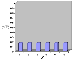

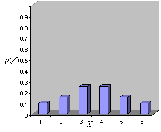
As you can see, the probability of each outcome is the same (1/6), indicating that this is a fair die. If the die was weighted toward middle values (3 and 4, for instance) rather than low and high values (such as 1 and 6), the graph might look more like the following.

The above probability distributions are discrete because only certain specific outcomes are possible. A probability distribution can be continuous, however, when an unbroken range of outcomes is possible. Let's say we have some random variable X that corresponds to an adult's height in inches. The probability distribution for this random variable might look like the following.
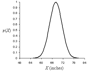

Calculating a probability of a particular outcome (such as that a particular adult's height is between 70 and 72 inches) is more complicated in the continuous case than it is in the discrete case, however. (Integral calculus, or at least a table of values, is needed to perform this calculation.)
Practice Problem: A loaded six-sided die has a 1/3 probability of rolling an even number and a 2/3 probability of rolling an odd number. Write a function for the probability of rolling n even numbers in a row followed by n odd numbers in a row.
Solution: The probability of rolling an even number in the first roll is 1/3. The probability of rolling two even numbers is then (1/3)2, and the probability of rolling three even numbers is (1/3)3. We can see a pattern in this: the probability of rolling n even numbers in a row is therefore (1/3)n. Likewise, the probability of rolling n odd numbers in a row is (2/3)n. To find the probability of rolling n even numbers and then n odd numbers, we simply multiply these two expressions. This is then the probability function that we are looking for. We'll call this function p(n), where n is a natural number.
p(n) = ![]()
We can simplify this expression as follows.
p(n) = ![]()
Algebra in Statistics
Likewise, algebra can play a critical role in statistics as well as probability (these two fields are interrelated and share a number of fundamental concepts). Algebra, for instance, allows us to write general formulas and expressions for fundamental parameters like the mean, variance, and standard deviation of a population (a set of data). Let's consider, for instance, the expression for the (unweighted) mean of a data set:
![]()
This expression simply states that we find the average by calculating the sum of all n data items (indexed using the variable i, which has no relation to the complex number i = ![]() ), which we then divide by n. Thus, if we want to calculate the mean of the data set {1, 4, 6, 6, 8, 9, 11, 15}, we do the following:
), which we then divide by n. Thus, if we want to calculate the mean of the data set {1, 4, 6, 6, 8, 9, 11, 15}, we do the following:
![]()
The above example illustrates calculation of a mean for a discrete data set. Means (and other statistical parameters) for continuous data sets can also be calculated, but these calculations require more sophisticated mathematical tools (such as integral calculus).
Practice Problem: Find an expression for the variance of a data set.
Solution: The variance of a data set is the sum of the squared differences between each data item in the set and the mean of the set. (This applies only to the unweighted case where each data item counts to the same extent as every other data item.) We can write this expression as follows using the same symbolism that we used for the mean. In the expression below, m is the mean of the data set and n is the number of data items in that set.
![]()