The one-sample and two-sample Student's t-tests allow us to compare a sample mean with a known or predetermined population mean or to compare two sample means. If we wish to compare more than two sample groups, however, we must turn to a different method. One-way ANOVA provides such a method, allowing us to compare the means of three or more sample groups. In this article, we focus on the one-way ANOVA test statistic and how to use it to determine if several sample means deviate significantly from each other.

Key Terms

o         Analysis of variances (ANOVA)

o         One-way ANOVA

o         F-test

Objectives

o         Identify the test statistic for one-way ANOVA

o         Use one-way ANOVA to compare the means of multiple sample groups

Resources

o         A table of values for the Student's't distribution is available at http://www.itl.nist.gov/div898/handbook/eda/section3/eda3673.htm

Let's Begin!

Introduction to One-Way ANOVA

Our study of ANOVA will be limited to so-called one-way ANOVA, which involves comparison of samples on the basis of only one factor (just as t-tests only involved one factor). For instance, a manufacturing company might wish to compare the quality of several groups of products on the basis of a certain setting on a given machine. (In this case, the "factor" is product quality.) Such a comparison would be impossible using t-tests, which only allow examination of two groups (or products, in this case). Using one-way ANOVA, however, the company could compare quality for any number of product groups. Thus, one-way ANOVA adds another tool to our statistical toolbox that we have developed.

One-way ANOVA differs from the Student's t-test primarily in the test statistic, which involves calculation of variances between and among the groups (or samples) under test. Although a thorough derivation of this test statistic is beyond the scope of this article, we have developed a sufficient foundation in statistics to facilitate a basic understanding of the statistic.

As with the Student's t-tests that we studied in the preceding two articles, one-way ANOVA is based on several assumptions. If these assumptions do not apply in a given situation, the analysis will be flawed. Thus, careful consideration of the problem is always required (both for ANOVA and for Student's t-tests) to avoid blind (and erroneous) use of hypothesis testing.

As with the Student's t-tests, one-way ANOVA assumes that the data are normally distributed and that the data groups have equivalent population variances. (Note, then, that the samples need not necessarily have the same variance, although they should be similar if they are chosen properly.) Furthermore, proper use of ANOVA assumes that the samples are independent. Following our manufacturing example, groups of products are independent if the selection of products for one group does not have any bearing on the selection of products for another group.

One-Way ANOVA Procedure

The overall approach to ANOVA is essentially the same as that of the Student's t-test; we will apply the hypothesis testing procedure once more, but our test statistic and the critical value associated with that statistic will be different in this case. Our null hypothesis will once again be the following (or some similar formulation):

H₀ = The sample means do not vary significantly for the factor under test.

The alternative hypothesis is then, of course, the negation of this statement.

Ha = The sample means vary significantly for the factor under test.

As with any hypothesis test, we must also choose a significance level. Also, as before, values of α = 0.05 and α = 0.01 are typical.

We must now determine a test statistic that adequately takes the multiple sample groups into account. We'll assume that we have k sample groups, each of which has n samples (we make this latter assumption for simplicity at this point). Thus, for group 1, we have data {x₁₁, x₁₂, x₁₃,., x_1n}; for group 2, {x₂₁, x₂₂, x₂₃,., x_2n}; and so on. We identify a general data element as x_ji, where j is the group number (1 to k) and i is the data item number (from 1 to n) in that group.

We can calculate the overall sample mean across all groups by adding all the data values from every group and dividing by the total number of values. We'll call this "grand mean" . The formula for calculating the grand mean is expressed below. Note that because each of the k groups contains n values, the total number of values is kn.

Each individual group j has a mean defined as follows. This is simply the sample mean for group j.

As the name indicates, ANOVA involves analysis of variances. Let's use the definitions and nomenclature above to calculate some parameters along these lines. We start with the "variation between groups," which we label SS_B; note that this is variation, not variance. The variation is simply a sum of squares. In this case, we are calculating the sum of the squared differences between the group sample means and the grand mean. We also multiply by n, the number of samples in each group.

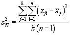
We can also calculate the total variation within the groups (SS_W). The expression for this case is more familiar--it is the sum of squares that we use in the sample variance formula, but it adds these sums across all groups.

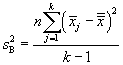
We can convert these variations into variances by dividing by the number of degrees of freedom in each case (this is the same thing we do when calculating a sample variance, for instance--in that case, the number of degrees of freedom is one less than the sample size). For the variation between groups (SS_B), the number of degrees of freedom is one less than the number of groups, or k – 1. For the variation within groups (SS_W), the number of degrees of freedom is the product of the number of groups and one less than the number of sample values-mathematically, k(n – 1). Let's then call the variance (technically, the "mean square") between groups and the variance (or "mean square") within groups. Then,

We can use these variances to calculate a test statistic, which is called the F-test. The test statistic F is expressed below in terms of the formulas above:

Although we followed a simpler approach to this statistic wherein the number of values in each sample group is equal to n, we can also calculate F for the more general case wherein the number of values in each sample group varies (we'll call n_j the number of values in each group j). These more general formulas for and are given below.

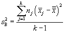
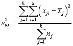
The formula for F remains the same.

The F statistic is then a ratio of variances. If the variance between groups is similar to the variance within groups, F will be relatively low. On the other hand, if the variance between groups is large compared with the variance within groups, then F will be relatively high. In the first case, the F-test is more likely to support the null hypothesis, whereas it is less likely to do so in the second case.

Of course, we also need a critical value with which to compare our test statistic. As with the t-test and chi-square statistics, these critical values are available in tables. The tables involve more parameters, so they are not arranged in precisely the same manner as those of the Student's't and chi-square statistics. In this case, the each table has one associated significance level, with the vertical axis usually associated with the number of degrees of freedom of the denominator in the F statistic and the horizontal axis usually associated with the number of degrees of freedom in the numerator of the F statistic. In our case, the number of degrees of freedom in the denominator is k(n – 1) (this is for the case where n is constant across all groups), and the number of degrees of freedom in the numerator is k – 1. Using specific values and a determined significance level, we can find the critical value and then use it to complete the hypothesis testing procedure in the usual manner.

The following practice problem illustrates the use of ANOVA and the F-test to determine whether the means of a few sample groups deviate significantly from one another.

Practice Problem: Determine whether the sample means of the three data groups below deviate in a statistically significant manner (assume a significance level of 0.05).

Solution: Since we are analyzing three groups, we can use ANOVA to determine if the sample means deviate significantly. First, note that the individual group means are the following:

Our null hypothesis is that these means do not vary in a statistically significant manner. We'll now use hypothesis testing by way of the F-test to check this statement to a significance level of 0.05.

The grand mean of all the data is

Since each group contains five values, we can use the simpler variance formulas.

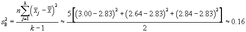
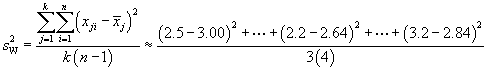
The F statistic is then

We must now determine the critical value. The number of degrees of freedom in the numerator of the F value is k – 1 = 2, and the number of degrees of freedom in the denominator is k(n – 1) = 12. Using the tables, we can find c for α = 0.05:

Because F < c, we can proceed on the assumption that the null hypothesis is correct.