Key Terms
o Correlation
o Correlation coefficient
o Pearson's correlation
Objectives
o Understand how variance can be used to define a statistic that measures the linear relationship between variables
o Use the correlation coefficient to quantify the correlation between two variables
Let's Begin!
In our discussion of cross tabulations, we often wanted to determine whether two variables in a data set were related in some manner. The chi-square statistic allowed us to test hypotheses in this regard--thus, we were able to state, to a certain specified statistical significance, that the variables did or did not have some kind of relationship. Although this hypothesis testing procedure for cross tabulations is indeed helpful, it does not quantify the degree to which the two variables are related. In this article, we will consider such a method of quantifying the relationship between two statistical variables: correlation.
Calculating the Correlation Coefficient
As mentioned, correlation measures the degree to which two variables are linearly related. The correlation coefficient (sometimes called Pearson's correlation, among other names) is a quantity that characterizes correlation numerically. To help define this value, recall from our discussion of multivariate data that we defined the covariance of two variables, ![]() , as follows.
, as follows.
![]()
Also, recall that the variance of a single variable X is the same as the covariance where X takes the place of both variables:
![]()
Using these expressions, we defined the covariance matrix as follows.

We can also define symbols to represent the summations contained in these covariances: ssXY, ssXX, and ssYY. The ss portion simply means "sum of squared values."
![]()
![]()
![]()
Note that these values are the same as the covariances without the leading coefficient involving N. (In other words, ![]() and so on.) These expressions are sometimes used in expressions involving regression and correlation.
and so on.) These expressions are sometimes used in expressions involving regression and correlation.
The covariance of two variables expresses how one variable varies with respect to another. Naturally, the covariance could then serve as a foundation for quantifying correlation. We can therefore use the expressions above to define the correlation coefficient, which we will label ρ.
![]()
Also, note that the standard deviations σX and σY are simply the square roots of the respective covariances (or simply variances) ![]() and
and ![]() . Thus, the correlation coefficient is a normalized form of the covariance,
. Thus, the correlation coefficient is a normalized form of the covariance, ![]() . We can also write the correlation coefficient in terms of our ss expressions.
. We can also write the correlation coefficient in terms of our ss expressions.

![]()
Several points regarding the correlation coefficient are noteworthy. First, the correlation coefficient, ρ, requires that the standard deviations σX and σY both be nonzero (in other words, all the X values in the data set cannot be the same, and neither can all the y values. Furthermore, ρ varies from –1 to 1, where 0 indicates no correlation, 1 indicates perfect linear correlation (with a positive line slope), and –1 indicates perfect linear correlation (with a negative line slope). We will further discuss these aspects of correlation when we treat regression analysis; for now, suffice it to say that the absolute value of the correlation coefficient (![]() ) varies from 0 (no correlation) to 1 (perfect correlation). (A proof that the correlation coefficient is limited to the range of –1 to 1 is beyond the scope of this article, but such a proof can be performed.)
) varies from 0 (no correlation) to 1 (perfect correlation). (A proof that the correlation coefficient is limited to the range of –1 to 1 is beyond the scope of this article, but such a proof can be performed.)
To be sure, as you may have noted, calculating the correlation coefficient can be tedious--computers are usually necessary for large data sets. Nevertheless, for small data sets, such computations are possible by hand. The following note about one pitfall associated with using correlation includes an example of how to calculate the correlation coefficient. A practice problem follows this brief discussion.
A Note of Caution about Correlation
If you have studied statistics in any depth, you may have heard the statement (or a similar statement), "correlation does not imply causation." The concept embodied in this statement is critical to properly interpreting correlation results. Although two variables in a data set might be highly correlated, we are not necessarily justified in assuming that this correlation indicates some causal dependence. For instance, consider the following age versus income (in thousands) data for a group of employees.

A relationship between age and income is apparent by inspection--older employees generally make more than younger employees (although this is clearly not always the case, meaning that the variables are not perfectly correlated). We can calculate the correlation coefficient to quantify how well the variables are related as follows, where the X variable is age (in years) and the Y variable is income (in thousands of dollars). First, we calculate the mean vector. (Note that for simplicity, we will assume the data set corresponds to a population rather than a sample.)
![]()
![]()
![]()
We can now calculate the covariance matrix.
![]()
![]()
![]()
![]()

At this point, we have everything we need to calculate ρ.
![]()
This result indicates that age and income are correlated to a significant degree (in the linear sense with a positive slope). By inspection, we can see that individuals with greater age clearly tend to have a higher income. Nevertheless, this does not mean that income is necessarily causally dependent on age. That is to say, although those with greater age tend to have a higher income, the cause of that higher income is not age. For example, older individuals may have a more developed skill set that leads to higher income, or they may have more experience in some area, thereby making them more valuable to an employer. Some other factor or factors may be involved as well. But a younger person who has the necessary experience, skill set, or other attribute may well be able to earn the same income as an older individual, thus indicating that although age and income are correlated, they do not share a causal connection.
From this example, we see that although correlation can be a helpful quantity in analyzing a data set, it must be interpreted carefully. Reaching invalid conclusions on the basis of data correlation is easy and tempting, but it must be avoided. Other information, in addition to correlation, is required to prove a causal connection. Nevertheless, correlation can still be helpful, when combined with other facts, in building a case for causality. Thus, in either case, correlation must always be interpreted and used with care, as with statistical value.
Practice Problem: Quantify how well the two variables in the following population data set are correlated.
|
Speed |
Acceleration |
|
46 |
12 |
|
52 |
14 |
|
53 |
17 |
|
54 |
18 |
|
59 |
17 |
|
62 |
22 |
Solution: Similar data appeared in our discussion of multivariate data in a previous article. Note that the scatterplot shows an apparent relationship between the two variables.
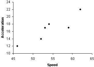
Let's quantify this relationship using the correlation coefficient. First, we'll calculate the mean vector.
![]()
![]()
![]()
Now, calculate the covariance matrix.
![]()
![]()
![]()
![]()

Finally, we can calculate the correlation coefficient.
![]()
Note that even though speed is closely correlated with acceleration, we do not have enough information to state whether one is causally related to the other. Thus, the best we can say is that the variables are well correlated--we cannot say that one causes another.
Other Correlation Values
Although we will not discuss them further here, other methods of quantifying correlation are available. The preceding discussion of Pearson's correlation coefficient covers one important method of calculating correlation; this method is useful in, for instance, linear regression analysis.


